| Title: | General Bivariate Copula Theory and Many Utility Functions |
| Version: | 2.2.11 |
| Date: | 2025-11-02 |
| Description: | Extensive functions for bivariate copula (bicopula) computations and related operations for bicopula theory. The lower, upper, product, and select other bicopula are implemented along with operations including the diagonal, survival copula, dual of a copula, co-copula, and numerical bicopula density. Level sets, horizontal and vertical sections are supported. Numerical derivatives and inverses of a bicopula are provided through which simulation is implemented. Bicopula composition, convex combination, asymmetry extension, and products also are provided. Support extends to the Kendall Function as well as the Lmoments thereof. Kendall Tau, Spearman Rho and Footrule, Gini Gamma, Blomqvist Beta, Hoeffding Phi, Schweizer- Wolff Sigma, tail dependency, tail order, skewness, and bivariate Lmoments are implemented, and positive/negative quadrant dependency, left (right) increasing (decreasing) are available. Other features include Kullback-Leibler Divergence, Vuong Procedure, spectral measure, and Lcomoments for fit and inference, Lcomoment ratio diagrams, maximum likelihood, and AIC, BIC, and RMSE for goodness-of-fit. |
| Maintainer: | William Asquith <william.asquith@ttu.edu> |
| Repository: | CRAN |
| Depends: | R (≥ 4.0.0) |
| Imports: | lmomco, mvtnorm, randtoolbox |
| Suggests: | copula |
| License: | GPL-2 |
| NeedsCompilation: | no |
| Packaged: | 2025-11-02 21:30:13 UTC; wasquith |
| Author: | William Asquith  [aut, cre]
 |
| Date/Publication: | 2025-11-03 06:10:15 UTC |
Basic Theoretical Copula, Empirical Copula, and Various Utility Functions
Description
The copBasic package is oriented around bivariate copula theory and mathematical operations closely follow the recommended texts of Nelsen (2006) and Joe (2014) as well as select other references. Another recommended text is Salvadori et al. (2007) and Hofert et al. (2018) and are cited herein, but about half of that excellent book concerns univariate applications. The primal objective of copBasic is to provide a study of numerous results shown by authoritative texts on copulas. It is intended that the package will help other copula students in self study, potential course work, and applied circumstances.
Notes on copulas that are supported. The author has focused on pedagogical aspects of copulas, and this package is a diary of sorts that began in fall 2008. Originally, the author did not implement many copulas in the copBasic in order to deliberately avoid redundancy to that support such as it exists on the R CRAN. Though as time has progressed, other copulas have been added based on needs of a user community, needs to show some concepts in the general theory, or test algorithms. For example, the Clayton copula (CLcop) was a late arriving addition the package (c.2017), which was added to assist a specific user; the Frank copula (FRcop was added in December 2024 because of an inquiry on using copBasic for vine copula (see vine example under FRcop). The Normal (NORMcop), Marshall–Olkin (MOcop), and t-Student copulas (Tcop) were added in summer 2025 because of an inquiry on meanings and interpretive properties of L-comoments.
The language and vocabulary of copulas are formidable even within the realm of bivariate or bicopula as design basis for the package. Often “vocabulary” words are often emphasized in italics, which is used extensively and usually near the opening of function-by-function documentation to identify vocabulary words, such as survival copula (see surCOP). This syntax tries to mimic and accentuate the terminology in Nelsen (2006), Joe (2014), and generally most other texts. Italics are used to draw connections between concepts.
In conjunction with the summary of functions in copBasic-package, the extensive cross referencing to functions and expansive keyword indexing should be beneficial. The author had no experience with copulas prior to a chance happening upon Nelsen (2006) in c.2008. The copBasic package is a personal tour de force in self-guided learning. Over time, this package and user's manual have been helpful to many others.
Helpful Navigation of Copulas Implemented in the copBasic Package
Some entry points to the copulas implemented are listed in the Table of Copulas:
| Name | Symbol | Function | Concept |
| Lower-bounds copula | \mathbf{W}(u,v) | W | copula |
| Independence copula | \mathbf{\Pi}(u,v) | P | copula |
| Upper-bounds copula | \mathbf{M}(u,v) | M | copula |
| Fréchet Family copula | \mathbf{FF}(u,v) | FRECHETcop | copula |
| Ali–Mikhail–Haq copula | \mathbf{AMH}(u,v) | AMHcop | copula |
| Clayton copula | \mathbf{CL}(u,v) | CLcop | copula |
| Copula of uniform circle | \mathbf{CIRC}(u,v) | CIRCcop | copula |
| Farlie–Gumbel–Morgenstern (generalized) | \mathbf{FGM}(u,v) | FGMcop | copula |
| Frank | \mathbf{FR}(u,v) | FRcop | copula |
| Galambos copula | \mathbf{GL}(u,v) | GLcop | copula |
| Gumbel–Hougaard copula | \mathbf{GH}(u,v) | GHcop | copula |
| Hairpin copula | \mathbf{HAIRPIN(u,v)} | HAIRPINcop | copula |
| Hüsler–Reiss copula | \mathbf{HR}(u,v) | HRcop | copula |
| Joe B5 (the “Joe”) copula | \mathbf{B5}(u,v) | JOcopB5 | copula |
| Joe–Ma copula | \mathbf{JOMA}(u,v) | JOMAcop | copula |
| Marshall–Olkin copula | \mathbf{MO}(u,v) | MOcop | copula |
| Nelsen eq.4-2-12 copula | \mathbf{N4212cop}(u,v) | N4212cop | copula |
| Nelsen eq.4-2-20 copula | \mathbf{N4220cop}(u,v) | N4220cop | copula |
| Nelsen eq.4-2-20 copula (reflected) | \mathbf{rN4220cop}(u,v) | rN4220cop | copula |
Normal copula (refer also to Tcop) | \mathbf{NORM}(u,v) | NORMcop | copula |
| Ordinal Sums by Copula | \mathbf{C}_\mathcal{J}(u,v) | ORDSUMcop | copula |
| Ordinal Sums by W-Copula | \mathbf{C}_\mathcal{J}(u,v) | ORDSUWcop | copula |
| Pareto copula | \mathbf{PA}(u,v) | PAcop | copula |
| Plackett copula | \mathbf{PL}(u,v) | PLcop | copula |
| PSP copula | \mathbf{PSP}(u,v) | PSP | copula |
| Raftery copula | \mathbf{RF}(u,v) | RFcop | copula |
| Rayleigh copula | \mathbf{RAY}(u,v) | RAYcop | copula |
| g-EV copula (Gaussian extreme value) | \mathbf{gEV}(u,v) | gEVcop | copula |
| t-EV copula (t-distribution extreme value) | \mathbf{tEV}(u,v) | tEVcop | copula |
t-Student copula (refer also to NORMcop) | \mathbf{T}(u,v) | Tcop | copula |
A few comments on notation herein are needed. A bold math typeface is used to represent a copula function or family such as \mathbf{\Pi} (see P) for the independence copula. The syntax \mathcal{R}\times\mathcal{R} \equiv \mathcal{R}^2 denotes the orthogonal domain of two real numbers, and [0,1]\times [0,1] \equiv \mathcal{I}\times\mathcal{I} \equiv \mathcal{I}^2 denotes the orthogonal domain on the unit square of probabilities. Limits of integration [0,1] or [0,1]^2 involving copulas are thus shown as \mathcal{I} and \mathcal{I}^2, respectively.
Random variables X and Y respectively denote the horizontal and vertical directions in \mathcal{R}^2. Their probabilistic counterparts are uniformly distributed random variables on [0, 1], are respectively denoted as U and V, and necessarily also are the respective directions in \mathcal{I}^2 (U denotes the horizontal, V denotes the vertical). Often realizations of these random variables are respectively x and y for X and Y and u and v for U and V. There is an obvious difference between nonexceedance probability F and its complement, which is exceedance probability defined as 1-F. Both u and v herein are in nonexceedance probability. Arguments to many functions herein are u = u and v = v and are almost exclusively nonexceedance but there are instances for which the probability arguments are u = 1 - u = u' and v = 1 - v = v'.
Bivariate Association — Several of the functions listed above are measures of bivariate association. Two of the measures (Kendall Tau, tauCOP; Spearman Rho, rhoCOP) are widely known. R provides native support for their sample estimation of course (stats::cor()), but each function can be used to call the cor() function for parallelism to the other measures of this package. The other measures (Blomqvist Beta, Gini Gamma, Hoeffding Phi, Schweizer–Wolff Sigma, Spearman Footrule) support sample estimation by specially formed calls to their respective functions: blomCOP, giniCOP, hoefCOP, wolfCOP, and footCOP. Gini Gamma (giniCOP) documentation (also joeskewCOP) shows extensive use of theoretical and sample computations for these and other functions.
Helpful Navigation of the copBasic Package
Some other entry points into the package are listed in the following table:
| Name | Symbol | Function | Concept |
| Copula | \mathbf{C}(u,v) | COP | copula theory |
\cdots | \mathbf{C}(u,v) | COP(..., reflect=*) | reflection |
\cdots | \mathbf{C}(u,v) | COP(..., reflect=*) | rotation |
| Survival copula | \hat{\mathbf{C}}(u',v') | surCOP | copula theory |
| Joint survival function | \overline{\mathbf{C}}(u,v) | surfuncCOP | copula theory |
| Co-copula | \mathbf{C}^\star(u',v') | coCOP | copula theory |
| Dual of a copula | \tilde{\mathbf{C}}(u,v) | duCOP | copula theory |
| Primary copula diagonal | \delta(t) | diagCOP | copula theory |
| Secondary copula diagonal | \delta^\star(t) | diagCOP | copula theory |
| Inverse copula diagonal | \delta^{(-1)}(f) | diagCOPatf | copula theory |
| Joint probability | {-}{-} | jointCOP | copula theory |
| Bivariate L-moments | \delta^{[\ldots]}_{k;\mathbf{C}} | bilmoms and lcomCOP | bivariate moments |
| Bivariate L-comoments | \tau^{[\ldots]}_{k;\mathbf{C}} | bilmoms and lcomCOP | bivariate moments |
| Blomqvist Beta | \beta_\mathbf{C} | blomCOP | bivariate association |
| Gini Gamma | \gamma_\mathbf{C} | giniCOP | bivariate association |
| Hoeffding Phi | \Phi_\mathbf{C} | hoefCOP | bivariate association |
| Nu-Skew | \nu_\mathbf{C} | nuskewCOP | bivariate moments |
| Nu-Star (skew) | \nu^\star_\mathbf{C} | nustarCOP | bivariate moments |
| Lp distance to independence | \Phi_\mathbf{C} \rightarrow L_p | LpCOP | bivariate association |
| Permutation-Mu | \mu_{\infty\mathbf{C}}^\mathrm{permsym} | LzCOPpermsym | permutation asymmetry |
| Kendall Tau | \tau_\mathbf{C} | tauCOP | bivariate association |
| Kendall Measure | K_\mathbf{C}(z) | kmeasCOP | copula theory |
| Kendall Function | F_K(z) | kfuncCOP | copula theory |
Kendall Function (d-\mathbf{P}) | F_K(z; \mathbf{P}_d) | kfuncCOP_Pd | copula theory |
| Inverse Kendall Function | F_K^{(-1)}(z) | kfuncCOPinv | copula theory |
An L-moment of F_K(z) | \lambda_r(F_K) | kfuncCOPlmom | L-moment theory |
L-moments of F_K(z) | \lambda_r(F_K) | kfuncCOPlmoms | L-moment theory |
| Semi-correlations (negatives) | \rho_N^{-}(a) | semicorCOP | bivariate tail association |
| Semi-correlations (positives) | \rho_N^{+}(a) | semicorCOP | bivariate tail association |
| Spearman Footrule | \psi_\mathbf{C} | footCOP | bivariate association |
| Spearman Rho | \rho_\mathbf{C} | rhoCOP | bivariate association |
| Schweizer–Wolff Sigma | \sigma_\mathbf{C} | wolfCOP | bivariate association |
| Density of a copula | c(u,v) | densityCOP | copula density |
| Density visualization | {-}{-} | densityCOPplot | copula density |
| Empirical copula | \mathbf{C}_n(u,v) | EMPIRcop | copula |
| Empirical simulation | {-}{-} | EMPIRsim | copula simulation |
| Empirical simulation | {-}{-} | EMPIRsimv | copula simulation |
| Empirical copulatic surface | {-}{-} | EMPIRgrid | copulatic surface |
| Parametric copulatic surface | {-}{-} | gridCOP | copulatic surface |
| Parametric simulation | {-}{-} | simCOP or rCOP | copula simulation |
| Parametric simulation | {-}{-} | simCOPmicro | copula simulation |
| Maximum likelihood | \mathcal{L}(\Theta_d) | mleCOP | copula fitting |
| Akaike information criterion | \mathrm{AIC}_\mathbf{C} | aicCOP | goodness-of-fit |
| Bayesian information crit. | \mathrm{BIC}_\mathbf{C} | bicCOP | goodness-of-fit |
| Root mean square error | \mathrm{RMSE}_\mathbf{C} | rmseCOP | goodness-of-fit |
| Another goodness-of-fit | T_n | statTn | goodness-of-fit |
Goodness-of-fit — Concerning goodness-of-fit and although not quite the same as copula properties (such as “correlation”) per se as the coefficients aforementioned in the prior paragraph, three goodness-of-fit metrics of a copula compared to the empirical copula, which are all based the mean square error (MSE), are aicCOP, bicCOP, and rmseCOP. This triad of functions is useful for making decisions on whether a copula is more favorable than another to a given dataset. However, because they are genetically related by using MSE and if these are used for copula fitting by minimization, the fits will be identical. A statement of “not quite the same” is made because the previously described copula properties are generally defined as types of deviations from other copulas (such as P). Another goodness-of-fit statistic is statTn, which is based on magnitude summation of fitted copula difference from the empirical copula. These four (aicCOP, bicCOP, rmseCOP, and statTn) collectively are relative simple and readily understood measures. These bulk sample statistics are useful, but generally thought to not capture the nuances of tail behavior (semicorCOP and taildepCOP might be useful).
Bivariate Skewness and L-comoments — Bivariate skewness measures are supported in the functions joeskewCOP (nuskewCOP and nustarCOP) and uvlmoms (uvskew). Extensive discussion and example computations of bivariate skewness are provided in the joeskewCOP documentation. Lastly, so-called bivariate L-moments and bivariate L-comoments of a copula are directly computable in bilmoms (though that function using Monte Carlo integration is deprecated) and lcomCOP (direct numerical integration). Function lcomCOP is the theoretical counterpart to the sample L-comoments provided in the lmomco package by lmomco::lcomoms2() function. Parameter estimation by L-comoments is demonstrated for the MOcop under its Examples and for a potentially complex composite1COP within Examples of lcomCOP. Demonstrations of L-comoment ratio diagrams and construction methods for various copula is seen in Examples within LCOMDIA_ManyCops (a collection of vary many 1-parameter copula driven by Spearman Rho, rhoCOP), LCOMDIA_GH2cop (2-parameter Gumbel–Hougaard copula, GHcop), LCOMDIA_GH3cop (3-parameter Gumbel–Hougaard copula, GHcop), and ORDSUMcop (ordinal sums of M-copula).
Conditional Simulation — Random simulation methods by several functions are listed in the previous table (simCOPmicro, simCOP). The copBasic package explicitly uses only conditional simulation also known as the conditional distribution method for random variate generation following Nelsen (2006, pp. 40–41). The numerical derivatives (derCOP and derCOP2) and their inversions (derCOPinv and derCOPinv2) (next table) represent the foundation of the conditional simulation. There are other methods in the literature and available in other R packages, and a comparison of some methods is made in the Examples section of the Gumbel–Hougaard copula (GHcop).
Several functions in copBasic make the distinction between V with respect to (wrt) U and U wrt V, and a guide for the nomenclature involving wrt distinctions is listed in the following table:
| Name | Symbol | Function | Concept |
| Copula inversion | V wrt U | COPinv | copula operator |
| Copula inversion | U wrt V | COPinv2 | copula operator |
| Copula derivative | \delta \mathbf{C}/\delta u | derCOP | copula operator |
| Copula derivative | \delta \mathbf{C}/\delta v | derCOP2 | copula operator |
| Copula derivative inversion | V wrt U | derCOPinv | copula operator |
| Copula derivative inversion | U wrt V | derCOPinv2 | copula operator |
| Joint curves | t \mapsto \mathbf{C}(u=U, v) | joint.curvesCOP | copula theory |
| Joint curves | t \mapsto \mathbf{C}(u, v=V) | joint.curvesCOP2 | copula theory |
| Level curves | t \mapsto \mathbf{C}(u=U, v) | level.curvesCOP | copula theory |
| Level curves | t \mapsto \mathbf{C}(u, v=V) | level.curvesCOP2 | copula theory |
| Level set | V wrt U | level.setCOP | copula theory |
| Level set | U wrt V | level.setCOP2 | copula theory |
| Median regression | V wrt U | med.regressCOP | copula theory |
| Median regression | U wrt V | med.regressCOP2 | copula theory |
| Quantile regression | V wrt U | qua.regressCOP | copula theory |
| Quantile regression | U wrt V | qua.regressCOP2 | copula theory |
| Copula section | t \mapsto \mathbf{C}(t,a) | sectionCOP | copula theory |
| Copula section | t \mapsto \mathbf{C}(a,t) | sectionCOP | copula theory |
The previous two tables do not list all of the myriad of special functions to support similar operations on empirical copulas. All empirical copula operators and utilities are prepended with EMPIR in the function name. An additional note concerning package nomenclature is that an appended “2” to a function name indicates U wrt V (e.g. EMPIRgridderinv2 for an inversion of the partial derivatives \delta \mathbf{C}/\delta v across the grid of the empirical copula).
Some additional functions to compute often salient features or characteristics of copulas or bivariate data, including functions for bivariate inference or goodness-of-fit, are listed in the following table:
| Name | Symbol | Function | Concept |
| Left-tail decreasing | V wrt U | isCOP.LTD | bivariate association |
| Left-tail decreasing | U wrt V | isCOP.LTD | bivariate association |
| Right-tail increasing | V wrt U | isCOP.RTI | bivariate association |
| Right-tail increasing | U wrt V | isCOP.RTI | bivariate association |
| Pseudo-polar representation | (\widehat{S},\widehat{W}) | psepolar | extremal dependency |
| Tail concentration function | q_\mathbf{C}(t) | tailconCOP | bivariate tail association |
| Tail (lower) dependency | \lambda^L_\mathbf{C} | taildepCOP | bivariate tail association |
| Tail (upper) dependency | \lambda^U_\mathbf{C} | taildepCOP | bivariate tail association |
| Tail (lower) order | \kappa^L_\mathbf{C} | tailordCOP | bivariate tail association |
| Tail (upper) order | \kappa^U_\mathbf{C} | tailordCOP | bivariate tail association |
| Neg'ly quadrant dependency | NQD | isCOP.PQD | bivariate association |
| Pos'ly quadrant dependency | PQD | isCOP.PQD | bivariate association |
| Permutation symmetry | \mathrm{permsym} | isCOP.permsym | copula symmetry |
| Radial symmetry | \mathrm{radsym} | isCOP.radsym | copula symmetry |
| Skewness (Joe, 2014) | \eta(p; \psi) | uvskew | bivariate skewness |
| Kullback–Leibler Divergence | \mathrm{KL}(f \mid g) | kullCOP | bivariate inference |
| KL sample size | n_{f\!g} | kullCOP | bivariate inference |
| The Vuong Procedure | {-}{-} | vuongCOP | bivariate inference |
| Spectral measure | H(w) | spectralmeas | extremal dependency inference |
| Stable tail dependence | \widehat{l}(x,y) | stabtaildepf | extremal dependency inference |
| L-comoments (samp. distr.) | {-}{-} | lcomCOPpv | experimental bivariate inference |
The Table of Probabilities that follows lists important relations between various joint probability concepts, the copula, nonexceedance probabilities u and v, and exceedance probabilities u' and v'. A compact summary of these probability relations has obvious usefulness. The notation [\ldots, \ldots] is to read as [\ldots \mathrm{\ and\ } \ldots], and the [\ldots \mid \ldots] is to be read as [\ldots \mathrm{\ given\ } \ldots].
| Probability | and | Symbol Convention |
\mathrm{Pr}[\,U \le u, V \le v\,] | = | \mathbf{C}(u,v) — The copula, COP |
\mathrm{Pr}[\,U > u, V > v\,] | = | \hat{\mathbf{C}}(u',v') — The survival copula, surCOP |
\mathrm{Pr}[\,U \le u, V > v\,] | = | u - \mathbf{C}(u,v') |
\mathrm{Pr}[\,U > u, V \le v\,] | = | v - \mathbf{C}(u',v) |
\mathrm{Pr}[\,U \le u \mid V \le v\,] | = | \mathbf{C}(u,v)/v |
\mathrm{Pr}[\,V \le v \mid U \le u\,] | = | \mathbf{C}(u,v)/u |
\mathrm{Pr}[\,U \le u \mid V > v\,] | = | \bigl(u - \mathbf{C}(u,v)\bigr)/(1 - v) |
\mathrm{Pr}[\,V \le v \mid U > u\,] | = | \bigl(v - \mathbf{C}(u,v)\bigr)/(1 - u) |
\mathrm{Pr}[\,U > u \mid V > v\,] | = | \hat{\mathbf{C}}(u',v')/u' = \overline{\mathbf{C}}(u,v)/(1-u) |
\mathrm{Pr}[\,V > v \mid U > u\,] | = | \hat{\mathbf{C}}(u',v')/v' = \overline{\mathbf{C}}(u,v)/(1-v) |
\mathrm{Pr}[\,V \le v \mid U = u\,] | = | \delta \mathbf{C}(u,v)/\delta u — Partial derivative, derCOP |
\mathrm{Pr}[\,U \le u \mid V = v\,] | = | \delta \mathbf{C}(u,v)/\delta v — Partial derivative, derCOP2 |
\mathrm{Pr}[\,U > u \mathrm{\ or\ } V > v\,] | = | \mathbf{C}^\star(u',v') = 1 - \mathbf{C}(u',v') — The co-copula, coCOP |
\mathrm{Pr}[\,U \le u \mathrm{\ or\ } V \le v\,] | = | \tilde{\mathbf{C}}(u,v) = u + v - \mathbf{C}(u,v) — The dual of a copula, duCOP |
E[\,U \mid V = v\,] | = | \int_0^1 (1 - \delta \mathbf{C}(u,v)/\delta v)\,\mathrm{d}u — Expectation of U given V, EuvCOP |
E[\,V \mid U = u\,] | = | \int_0^1 (1 - \delta \mathbf{C}(u,v)/\delta u)\,\mathrm{d}v — Expectation of V given U, EvuCOP |
The function jointCOP has considerable demonstration in its Note section of the joint and and joint or relations shown through simulation and counting scenarios. Also there is a demonstration in the Note section of function duCOP on application of the concepts of joint and conditions, joint or conditions, and importantly joint mutually exclusive or conditions.
Copula Construction Methods
Permutation asymmetry (nonexchangability) can be added to (inserted in) a copula by breveCOP. One, two, or more copulas can be “composited,” “combined,” or “multiplied” in interesting ways to create highly unique bivariate relations and as a result, complex dependence structures can be formed. Such operations can often insert permutation asymmetry as well. To such an end, the package provides three main functions for copula composition: composite1COP composites a single copula with two compositing parameters (Khoudraji device with independence), composite2COP (Khoudraji device) composites two copulas with two compositing parameters, and composite3COP composites two copulas with four compositing parameters.
Two copulas also can be combined through a weighted convex combination using convex2COP with a single weighting parameter, and even N number of copulas can be combined by weights using convexCOP. So-called “gluing” two copula by a parameter is provided by glueCOP. Multiplication of two copulas to form a third is supported by prod2COP. All eight functions for compositing, combining, or multiplying copulas are compatible with joint probability simulation (simCOP), measures of association (e.g. \rho_\mathbf{C}), and presumably all other copula operations using copBasic features. Finally, ordinal sums of copula are provided by ORDSUMcop and ORDSUWcop as particularly interesting methods of combining copulas.
| No. of copulas | Combining Parameters | Function | Concept |
| 1 | \beta | breveCOP | adding permuation asymmetry |
| 1 | \alpha, \beta | composite1COP | copula combination |
| 1 | \alpha, \beta | khoudraji1COP | copula combination |
| 1 | \alpha, \beta | khoudrajiPCOP | copula combination |
| 2 | \alpha, \beta | composite2COP | copula combination |
| 2 | \alpha, \beta | khoudraji2COP | copula combination |
| 2 | \alpha, \beta, \kappa, \gamma | composite3COP | copula combination |
| 2 | \alpha, (1-\alpha) | convex2COP | weighted copula combination |
N | \omega_{i \in N} | convexCOP | weighted copula combination |
| 2 | \gamma | glueCOP | gluing of coupla |
| 2 | \bigl(\mathbf{C}_1 \ast \mathbf{C}_2 \bigr) | prod2COP | copula multiplication |
N | \mathbf{C}_{\mathcal{J}i} for \mathcal{J}_{i \in N} partitions | ORDSUMcop | M-ordinal sums of copulas |
N | \mathbf{C}_{\mathcal{J}i} for \mathcal{J}_{i \in N} partitions | ORDSUWcop | W-ordinal sums of copulas |
Useful Copula Relations by Visualization
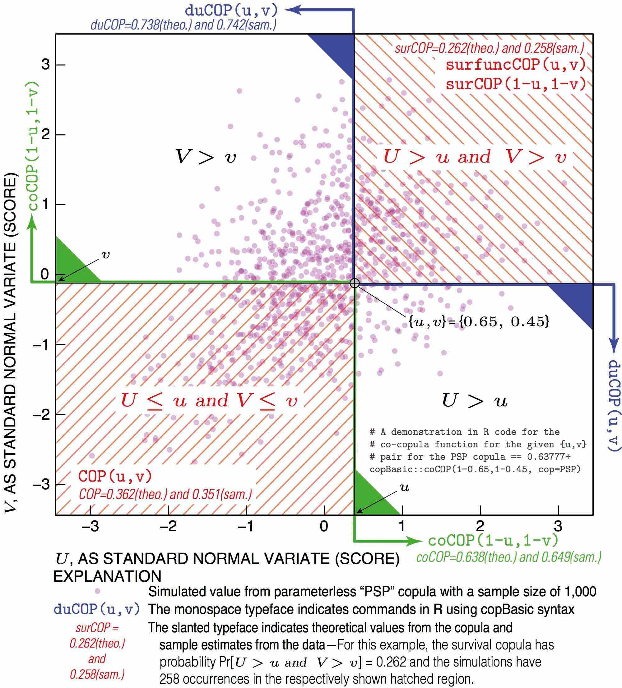
There are a myriad of relations amongst variables computable through copulas, and these were listed in the Table of Probabilities earlier in this documentation. There is a script located in the inst/doc directory of the copBasic sources titled CopulaRelations_BaseFigure_inR.txt. This script demonstrates, using the PSP copula, relations between the copula (COP), survival copula (surCOP), joint survival function of a copula (surfuncCOP), co-copula (coCOP), and dual of a copula function (duCOP). The script performs simulation and manual counts observations meeting various criteria in order to compute their empirical probabilities. The script produces a base figure, which after extending in editing software, is suitable for educational description and is provided at the end of this documentation.
A Review of “Return Periods” using Copulas
Study of natural hazards commonly use as annual return periods T in years, which are defined for a nonexceedance probability q as T = 1/(1-q). In bivariate analysis, there immediately emerge two types of return periods representing T_{q;\,\mathrm{coop}} and T_{q;\,\mathrm{dual}} conditions between nonexceedances of the two hazard sources (random variables) U and V. It is usual in many applications for T to be expressed equivalently as a probability q in common for both variables.
Incidentally, the \mathrm{Pr}[\,U > u \mid V > v\,] and \mathrm{Pr}[\,V > v \mid U > u\,] probabilities also are useful for conditional return period computations following Salvadori et al. (2007, pp. 159–160) but are not further considered here. Also the F_K(w) (Kendall Function or Kendall Measure of a copula) is the core tool for secondary return period computations (see kfuncCOP).
Let the copula \mathbf{C}(u,v; \Theta) for nonexceedances u and v be set for some copula family (formula) by a parameter vector \Theta. The copula family and parameters define the joint coupling (loosely meant the dependency/correlation) between hazards U and V. If “failure” occurs if either or both hazards U and V are at probability q threshold (u = v = 1 - 1/T = q) for T-year return period, then the real return period of failure is defined using either the copula \mathbf{C}(q,q; \Theta) or the co-copula \mathbf{C}^\star(q',q'; \Theta) for exceedance probability q' = 1 - q is
T_{q;\,\mathrm{coop}} = \frac{1}{1 - \mathbf{C}(q, q; \Theta)} = \frac{1}{\mathbf{C}^\star(1-q, 1-q; \Theta)}\mbox{\ and}
T_{q;\,\mathrm{coop}} \equiv \frac{1}{\mathrm{cooperative\ risk}}\mbox{.}
Or in words, the hazard sources collaborate or cooperate to cause failure. If failure occurs, however, if and only if both hazards U and V occur simultaneously (the hazards must “dually work together” or be “conjunctive”), then the real return period is defined using either the dual of a copula (function) \tilde{\mathbf{C}}(q,q; \Theta), the joint survival function \overline{\mathbf{C}}(q,q;\Theta), or survival copula \hat{\mathbf{C}}(q',q'; \Theta) as
T_{q;\,\mathrm{dual}} = \frac{1}{1 - \tilde{\mathbf{C}}(q,q; \Theta)} = \frac{1}{\overline{\mathbf{C}}(q,q;\Theta)} = \frac{1}{\hat{\mathbf{C}}(q',q';\Theta)} \mbox{\ and}
T_{q;\,\mathrm{dual}} \equiv \frac{1}{\mathrm{complement\ of\ dual\ protection}}\mbox{.}
Numerical demonstration is informative. Salvadori et al. (2007, p. 151) show for a Gumbel–Hougaard copula (GHcop) having \Theta = 3.055 and T = 1,000 years (q = 0.999) that T_{q;\,\mathrm{coop}} = 797.1 years and that T_{q;\,\mathrm{dual}} = 1,341.4 years, which means that average return periods between “failures” are
T_{q;\,\mathrm{coop}} \le T \le T_{q;\,\mathrm{dual}}\mbox{\ and thus}
797.1 \le T \le 1314.4\mbox{\ years.}
With the following code, these bounding return-period values are readily computed and verified using the prob2T() function from the lmomco package along with copBasic functions COP (generic functional interface to a copula) and duCOP (dual of a copula):
  q <- lmomco::T2prob(1000)
  lmomco::prob2T(  COP(q,q, cop=GHcop, para=3.055)) #  797.110
  lmomco::prob2T(duCOP(q,q, cop=GHcop, para=3.055)) # 1341.438
An early source (in 2005) by some of those authors cited on p. 151 of Salvadori et al. (2007; their citation “[67]”) shows T_{q;\,\mathrm{dual}} = 798 years—a rounding error seems to have been committed. Finally and just for reference, a Gumbel–Hougaard copula having \Theta = 3.055 corresponds to an analytical Kendall Tau (see GHcop) of \tau \approx 0.673, which can be verified through numerical integration available from tauCOP as:
tauCOP(cop=GHcop, para=3.055, brute=TRUE) # 0.6726542
Thus, a “better understanding of the statistical characteristics of [multiple hazard sources] requires the study of their joint distribution” (Salvadori et al., 2007, p. 150).
Interaction of copBasic to the Copulas and Features of Other Packages
The copBasic package (c. 2008–11) was not originally intended to be a port of the numerous bivariate copulas or over re-implementation other bivariate copulas available in R, but in support of didactic and teaching efforts. Though as the package passed its 10th year in 2018, the original intent changed to a more generalized purpose as more copula were added and other features by request. It is useful to point out a demonstration showing an implementation of the Gaussian copula from the copula package, which is shown in the Note section of med.regressCOP in a circumstance of ordinary least squares linear regression compared to median regression of a copula as well as prediction limits of both regressions. Another demonstration in context of maximum pseudo-log-likelihood estimation of copula parameters is seen in the Note section mleCOP, and also see “API to the copula package” or “package copula (comparison to)” entries in the Index of this user manual.
Author(s)
William Asquith william.asquith@ttu.edu
References
Cherubini, U., Luciano, E., and Vecchiato, W., 2004, Copula methods in finance: Hoboken, NJ, Wiley, 293 p.
Hernández-Maldonado, V., Díaz-Viera, M., and Erdely, A., 2012, A joint stochastic simulation method using the Bernstein copula as a flexible tool for modeling nonlinear dependence structures between petrophysical properties: Journal of Petroleum Science and Engineering, v. 90–91, pp. 112–123.
Joe, H., 2014, Dependence modeling with copulas: Boca Raton, CRC Press, 462 p.
Hofert, M., Kojadinovic, I., Mächler, M., and Yan, J., 2018, Elements of copula modeling with R: Dordrecht, Netherlands, Springer.
Nelsen, R.B., 2006, An introduction to copulas: New York, Springer, 269 p.
Salvadori, G., De Michele, C., Kottegoda, N.T., and Rosso, R., 2007, Extremes in nature—An approach using copulas: Dordrecht, Netherlands, Springer, Water Science and Technology Library 56, 292 p.
Examples
## Not run:
  # Nelsen (2006, p. 75, exer. 3.15b) provides for a nice test of copBasic features.
  "mcdurv" <- function(u,v, theta) {
     ifelse(u > theta & u < 1-theta & v > theta & v < 1 - theta,
               return(M(u,v) - theta), # Upper bounds copula with a shift
               return(W(u,v)))         # Lower bounds copula
  }
  "MCDURV" <- function(u,v, para=NULL) {
     if(is.null(para))         stop("need theta")
     if(para < 0 | para > 0.5) stop("theta ! in [0, 1/2]")
     return(asCOP(u, v, f=mcdurv, para))
  }
  "afunc" <- function(t) { # a sample size = 1,000 hard wired
     return(cov(simCOP(n=1000, cop=MCDURV, para=t, ploton=FALSE, points=FALSE))[1,2])
  }
  set.seed(6234) # setup covariance based on parameter "t" and the "root" parameter
  print(uniroot(afunc, c(0, 0.5))) # "t" by simulation = 0.1023742
  # Nelsen reports that if theta approx. 0.103 then covariance of U and V is zero.
  # So, one will have mutually completely dependent uncorrelated uniform variables!

  # Let us check some familiar measures of association:
  rhoCOP( cop=MCDURV, para=0.1023742) # Spearman Rho = 0.005854481 (near zero)
  tauCOP( cop=MCDURV, para=0.1023742) # Kendall Tau  = 0.2648521
  wolfCOP(cop=MCDURV, para=0.1023742) # S & W Sigma  = 0.4690174 (less familiar)
  D <- simCOP(n=1000, cop=MCDURV, para=0.1023742) # Plot mimics Nelsen (2006, fig. 3.11)
  # L-comoments (matrices) measure high dimensional variable comovements
  # L-comoments (refer also to the lmomco package)
  lcomCOP(cop=MCDURV, para=0.1023742)
  lmomco::lcomoms2(simCOP(n=1000, cop=MCDURV, para=0.1023742), nmom=5)
  lmomco::lcomoms2(simCOP(n=1000, cop=MCDURV, para=0),   nmom=5) # Perfect neg. corr.
  lmomco::lcomoms2(simCOP(n=1000, cop=MCDURV, para=0.5), nmom=5) # Perfect pos. corr.
  # T2 (L-correlation), T3 (L-coskew), T4 (L-cokurtosis), and T5 matrices result. For
  # Theta = 0 or 0.5 see the matrix symmetry with a sign change for L-coskew and T5 on
  # the off diagonals (offdiags). See unities for T2. See near zero for offdiag terms
  # in T2 near zero. But then see that T4 off diagonals are quite different from those
  # for Theta 0.1024 relative to 0 or 0.5. As a result, T4 has captured a unique
  # property of U vs V.
## End(Not run)
The Ali–Mikhail–Haq Copula
Description
The Ali–Mikhail–Haq copula (Nelsen, 2006, pp. 92–93, 172) is
\mathbf{C}_{\Theta}(u,v) = \mathbf{AMH}(u,v) = \frac{uv}{1 - \Theta(1-u)(1-v)}\mbox{,}
where \Theta \in [-1,+1), where the right boundary,
\Theta = 1, can sometimes be considered valid according to Mächler (2014). The copula \Theta \rightarrow 0 becomes the independence copula (\mathbf{\Pi}(u,v); P), and the parameter \Theta is readily computed from a Kendall Tau (tauCOP) by
\tau_\mathbf{C} = \frac{3\Theta - 2}{3\Theta} -
                        \frac{2(1-\Theta)^2\log(1-\Theta)}{3\Theta^2}\mbox{,}
and by Spearman Rho (rhoCOP), through Mächler (2014), by
\rho_\mathbf{C} = \sum_{k=1}^\infty \frac{3\Theta^k}{{k + 2 \choose 2}^2}\mbox{.}
The support of \tau_\mathbf{C} is [(5 - 8\log(2))/3, 1/3] \approx [-0.1817258, 0.3333333] and the \rho_\mathbf{C} is [33 - 48\log(2), 4\pi^2 - 39] \approx [-0.2710647, 0.4784176], which shows that this copula has a limited range of dependency. The infinite summation is easier to work with than
Nelsen (2006, p. 172) definition of
\rho_\mathbf{C} = \frac{12(1+\Theta)}{\Theta^2}\mathrm{dilog}(1-\Theta)-
                        \frac{24(1-\Theta)}{\Theta^2}\log(1-\Theta)-
                        \frac{3(\Theta+12)}{\Theta}\mbox{,}
where the \mathrm{dilog(x)} is the dilogarithm function defined by
\mathrm{dilog}(x) = \int_1^x \frac{\log(t)}{1-t}\,\mathrm{d}t\mbox{.}
The integral version has more nuances with approaches toward \Theta = 0 and \Theta = 1 than the infinite sum version.
Usage
AMHcop(u, v, para=NULL, rho=NULL, tau=NULL, fit=c("rho", "tau"), ...)
Arguments
u |
Nonexceedance probability |
v |
Nonexceedance probability |
para |
A vector (single element) of parameters—the |
rho |
Optional Spearman Rho from which the parameter will be estimated and presence of |
tau |
Optional Kendall Tau from which the parameter will be estimated; |
fit |
If |
... |
Additional arguments to pass. |
Value
Value(s) for the copula are returned. Otherwise if tau is given, then the \Theta is computed and a list having
para |
The parameter |
tau |
Kendall Tau. |
and if para=NULL and tau=NULL, then the values within u and v are used to compute Kendall Tau and then compute the parameter, and these are returned in the aforementioned list.
Note
Mächler (2014) reports on accurate computation of \tau_\mathbf{C} and \rho_\mathbf{C} for this copula for conditions of \Theta \rightarrow 0 and in particular derives the following equation, which does not have \Theta in the denominator:
\rho_\mathbf{C} = \sum_{k=1}^{\infty} \frac{3\Theta^k}{{k+2 \choose 2}^2}\mbox{.}
The copula package provides a Taylor series expansion for \tau_\mathbf{C} for small \Theta in the copula::tauAMH(). This is demonstrated here between the implementation of \tau = 0 for parameter estimation in the copBasic package to that in the more sophisticated implementation in the copula package.
copula::tauAMH(AMHcop(tau=0)$para) # theta = -2.313076e-07
It is seen that the numerical approaches yield quite similar results for small \tau_\mathbf{C}, and finally, a comparison to the \rho_\mathbf{C} is informative:
  rhoCOP(AMHcop, para=1E-9)    # 3.333333e-10 (two nested integrations)
  copula:::.rhoAmhCopula(1E-9) # 3.333333e-10 (cutoff based)
  theta <- seq(-1,1, by=.0001)
  RHOa <- sapply(theta, function(t) rhoCOP(AMHcop, para=t))
  RHOb <- sapply(theta, function(t) copula:::.rhoAmhCopula(t))
  plot(10^theta, RHOa-RHOb, type="l", col=2)
The plot shows that the apparent differences are less than 1 part in 100 million—The copBasic computation is radically slower though, but rhoCOP was designed for generality of copula family.
Author(s)
W.H. Asquith
References
Joe, H., 2014, Dependence modeling with copulas: Boca Raton, CRC Press, 462 p.
Mächler, Martin, 2014, Spearman's Rho for the AMH copula—A beautiful formula: copula package vignette, accessed on April 7, 2018, at https://CRAN.R-project.org/package=copula under the vignette rhoAMH-dilog.pdf.
Nelsen, R.B., 2006, An introduction to copulas: New York, Springer, 269 p.
Pranesh, Kumar, 2010, Probability distributions and estimation of Ali–Mikhail–Haq copula: Applied Mathematical Sciences, v. 4, no. 14, p. 657–666.
See Also
Examples
## Not run:
  t <- 0.9 # The Theta of the copula and we will compute Spearman Rho.
  di <- integrate(function(t) log(t)/(1-t), lower=1, upper=(1-t))$value
  A <- di*(1+t) - 2*log(1-t) + 2*t*log(1-t) - 3*t # Nelsen (2007, p. 172)
  rho <- 12*A/t^2 - 3    # 0.4070369
  rhoCOP(AMHcop, para=t) # 0.4070369
  sum(sapply(1:100, function(k) 3*t^k/choose(k+2, 2)^2)) # Machler (2014)
  # 0.4070369 (see Note section, very many tens of terms are needed)
## End(Not run)

## Not run:
  layout(matrix(1:2, byrow=TRUE)) # Note: Kendall Tau is same on reversal.
  s <- 2; set.seed(s); nsim <- 10000
  UVn <- simCOP(nsim, cop=AMHcop, para=c(-0.9, "FALSE" ), col=4)
  mtext("Normal definition [default]") # '2nd' parameter could be skipped
  set.seed(s) # seed used to keep Rho/Tau inside attainable limits
  UVr <- simCOP(nsim, cop=AMHcop, para=c(-0.9, "TRUE"),   col=2)
  mtext("Reversed definition")
  AMHcop(UVn[,1], UVn[,2], fit="rho")$rho # -0.2581653
  AMHcop(UVr[,1], UVr[,2], fit="rho")$rho # -0.2570689
  rhoCOP(cop=AMHcop, para=-0.9)           # -0.2483124
  AMHcop(UVn[,1], UVn[,2], fit="tau")$tau # -0.1731904
  AMHcop(UVr[,1], UVr[,2], fit="tau")$tau # -0.1724820
  tauCOP(cop=AMHcop, para=-0.9)           # -0.1663313
## End(Not run)
Copula of Circular Uniform Distribution
Description
The Circular copula of the coordinates (x, y) of a point chosen at random on the unit circle (Nelsen, 2006, p. 56) is given by
\mathbf{C}_{\mathrm{CIRC}}(u,v) = \mathbf{M}(u,v) \mathrm{\ for\ }|u-v| > 1/2\mathrm{,}
\mathbf{C}_{\mathrm{CIRC}}(u,v) = \mathbf{W}(u,v) \mathrm{\ for\ }|u+v-1| > 1/2\mathrm{,\ and}
\mathbf{C}_{\mathrm{CIRC}}(u,v) = \frac{u+v}{2} - \frac{1}{4} \mathrm{\ otherwise\ }\mathrm{.}
The coordinates of the unit circle are given by
\mathbf{CIRC}(x,y) = \biggl(\frac{\mathrm{cos}\bigl(\pi(u-1)\bigr)+1}{2}, \frac{\mathrm{cos}\bigl(\pi(v-1)\bigr)+1}{2}\biggr)\mathrm{.}
Usage
CIRCcop(u, v, para=NULL, as.circ=FALSE, ...)
Arguments
u |
Nonexceedance probability |
v |
Nonexceedance probability |
para |
Optional parameter list argument that can contain the logical |
as.circ |
A logical, if true, to trigger the transformation |
... |
Additional arguments to pass, if ever needed. |
Value
Value(s) for the copula are returned.
Author(s)
W.H. Asquith
References
Nelsen, R.B., 2006, An introduction to copulas: New York, Springer, 269 p.
Examples
CIRCcop(0.5, 0.5) # 0.25 quarterway along the diagonal upward to right
CIRCcop(0.5, 1  ) # 0.50 halfway across in horizontal direction
CIRCcop(1  , 0.5) # 0.50 halfway across in  vertical  direction

## Not run:
  nsim <- 2000
  opts <- par(xpd=NA, las=1, lend=2, no.readonly=TRUE)
  rtheta <- runif(nsim, min=0, max=2*pi) # polar coordinate simulation
  XY <- data.frame(X=cos(rtheta)/2 + 1/2, Y=sin(rtheta)/2 + 1/2)
  plot(XY, lwd=0.8, col="lightgreen", xaxs="i", yaxs="i",
           xlab="X OF UNIT CIRCLE OR NONEXCEEDANCE PROBABILITY U",
           ylab="Y OF UNIT CIRCLE OR NONEXCEEDANCE PROBABILITY V")
  UV <- simCOP(nsim, cop=CIRCcop, lwd=0.8, col="salmon3", ploton=FALSE)
  theta <- 3/4*pi+0.1 # select a point on the upper left of the circle
  x <- cos(theta)/2 + 1/2; y <- sin(theta)/2 + 1/2 # coordinates
  H <- CIRCcop(x, y, as.circ=TRUE) # 0.218169  # Pr[X <= x & Y <= y]
  points(x, y, pch=16, col="forestgreen", cex=2)
  segments(0, y, x, y, lty=2, lwd=2, col="forestgreen")
  segments(x, 0, x, y, lty=2, lwd=2, col="forestgreen")
  Hemp1 <- sum(XY$X <= x & XY$Y <= y) / nrow(XY) # about 0.22 as expected
  u <- 1-acos(2*x-1)/pi; v <- 1-acos(2*y-1)/pi
  segments(0, v, u, v, lty=2, lwd=2, col="salmon3")
  segments(u, 0, u, v, lty=2, lwd=2, col="salmon3")
  points(u, v, pch=16, cex=2,        col="salmon3")
  arrows(x, y, u, v, code=2, lwd=2, angle=15) # arrow points from (X,Y) coordinate
  # specified by angle theta in radians on the unit circle to the corresponding
  # coordinate in (U,V) domain of uniform circular distribution copula
  Hemp2 <- sum(UV$U <= u & UV$V <= v) / nrow(UV) # about 0.22 as expected
  # Hemp1 and Hemp2 are about equal to each other and converge as nsim
  # gets very large, but the origin of the simulations to get to each
  # are different: (1) one in polar coordinates and (2) by copula.
  # Now, draw the level curve for the empirical Hs and as nsim gets large the two
  # lines will increasingly plot on top of each other.
  lshemp1 <- level.setCOP(cop=CIRCcop, getlevel=Hemp1, lines=TRUE, col="blue", lwd=2)
  lshemp2 <- level.setCOP(cop=CIRCcop, getlevel=Hemp2, lines=TRUE, col="blue", lwd=2)
  txt <- paste0("level curves for Pr[X <= x & Y <= y] and\n",
                "level curves for Pr[U <= u & V <= v],\n",
                "which equal each other as nsim gets large")
  text(0.52, 0.52, txt, srt=-46, col="blue"); par(opts) #
## End(Not run)

## Not run:
  # Nelsen (2007, ex. 3.2, p. 57) # Singular bivariate distribution with
  # standard normal margins that is not bivariate normal.
  U <- runif(500); V <- simCOPmicro(U, cop=CIRCcop)
  X  <- qnorm(U, mean=0, sd=1);    Y <- qnorm(V, mean=0, sd=1)
  plot(X,Y, main="Nelsen (2007, ex. 3.2, p. 57)", xlim=c(-4,4), ylim=c(-4,4),
            lwd=0.8, col="turquoise3")
  rug(X, side=1, col="salmon3", tcl=0.5)
  rug(Y, side=2, col="salmon3", tcl=0.5) #
## End(Not run)

## Not run:
  DX <- c(5, 5, -5, -5); DY <- c(5, 5, -5, -5); D <- 6; R <- D/2
  xylim <- c(-10, 10)
  plot(DX, DY, type="n", xlim=xylim, ylim=xylim, xlab="X", ylab="Y", las=1,
       xaxs="i", yaxs="i")
  for(i in seq_len(length(DX))) lines(rep(DX[i], 2), xylim, lwd=2, col="seagreen")
  for(i in seq_len(length(DY))) lines(xylim, rep(DY[i], 2), lwd=2, col="seagreen")
  for(i in seq_len(length(DX))) {
    for(j in seq_len(length(DY))) {
      UV <- simCOP(n=30, cop=CIRCcop, pch=16, col="darkgreen", cex=0.5, graphics=FALSE)
      points(UV[,1]-0.5, UV[,2]-0.5,  pch=16, col="darkgreen", cex=0.5)
      XY <- data.frame(X=DX[i]+sign(DX[i])*D*(cos(pi*(UV$U-1))+1)/2-sign(DX[i])*R,
                       Y=DY[j]+sign(DY[j])*D*(cos(pi*(UV$V-1))+1)/2-sign(DY[j])*R)
      points(XY, lwd=0.8, col="darkgreen")
    }
    lines(rep(DX[i]+R, 2), xylim, lty=2, col="seagreen")
    lines(rep(DX[i]-R, 2), xylim, lty=2, col="seagreen")
    lines(xylim, rep(DY[i]+R, 2), lty=2, col="seagreen")
    lines(xylim, rep(DY[i]-R, 2), lty=2, col="seagreen")
  } #
## End(Not run)

## Not run:
  para <- list(cop1=CIRCcop, para1=NULL, cop2=W, para2=NULL, alpha=0.8, beta=0.8)
  UV <- simCOP(n=2000, col="salmon3", cop=composite2COP, para=para)
  XY <- data.frame(X=(cos(pi*(UV$U-1))+1)/2, Y=(cos(pi*(UV$V-1))+1)/2)
  plot(XY, type="n", xlab=paste0("X OF CIRCULAR UNIFORM DISTRIBUTION OR\n",
                                 "NONEXCEEDANCE PROBABILITY OF U"),
                     ylab=paste0("Y OF CIRCULAR UNIFORM DISTRIBUTION OR\n",
                                 "NONEXCEEDANCE PROBABILITY OF V"))
  JK <- data.frame(U=1 - acos(2*XY$X - 1)/pi, V=1 - acos(2*XY$Y - 1)/pi)
  segments(x0=UV$U, y0=UV$V, x1=XY$X, y1=XY$Y, col="lightgreen", lwd=0.8)
  points(XY, lwd=0.8, col="darkgreen")
  points(JK, pch=16,  col="salmon3", cex=0.5)

  t <- seq(0.001, 0.999, by=0.001)
  t <- diagCOPatf(t, cop=composite2COP, para=para)
  AB <- data.frame(X=(cos(pi*(t-1))+1)/2, Y=(cos(pi*(t-1))+1)/2)
  lines(AB, lwd=4, col="seagreen") #
## End(Not run)
The Clayton Copula
Description
The Clayton copula (Joe, 2014, p. 168) is
\mathbf{C}_{\Theta}(u,v) = \mathbf{CL}(u,v) = \mathrm{max}\bigl[(u^{-\Theta}+v^{-\Theta}-1; 0)\bigr]^{-1/\Theta}\mbox{,}
where \Theta \in [-1,\infty), \Theta \ne 0. The copula, as \Theta \rightarrow -1^{+} limits, to the countermonotonicity coupla (\mathbf{W}(u,v); W), as \Theta \rightarrow 0 limits to the independence copula (\mathbf{\Pi}(u,v); P), and as \Theta \rightarrow \infty, limits to the comonotonicity copula (\mathbf{M}(u,v); M). The parameter \Theta is readily computed from a Kendall Tau (tauCOP) by \tau_\mathbf{C} = \Theta/(\Theta+2).
Usage
CLcop(u, v, para=NULL, tau=NULL, ...)
Arguments
u |
Nonexceedance probability |
v |
Nonexceedance probability |
para |
A vector (single element) of parameters—the |
tau |
Optional Kendall Tau; and |
... |
Additional arguments to pass. |
Value
Value(s) for the copula are returned. Otherwise if tau is given, then the \Theta is computed and a list having
para |
The parameter |
tau |
Kendall Tau. |
and if para=NULL and tau=NULL, then the values within u and v are used to compute Kendall Tau and then compute the parameter, and these are returned in the aforementioned list.
Author(s)
W.H. Asquith
References
Joe, H., 2014, Dependence modeling with copulas: Boca Raton, CRC Press, 462 p.
See Also
Examples
# Lower tail dependency of Theta = pi --> 2^(-1/pi) = 0.8020089 (Joe, 2014, p. 168)
taildepCOP(cop=CLcop, para=pi)$lambdaL # 0.80201
The Copula
Description
Compute the copula or joint distribution function through a copula as shown by Nelsen (2006, p. 18) is the joint probability
\mathrm{Pr}[U \le u, V \le v] = \mathbf{C}(u,v)\mbox{.}
The copula is an expression of the joint probability that both U \le u and V \le v.
A copula is a type of dependence function that permits straightforward characterization of dependence from independence. Joe (2014, p. 8) comments that “copula families are usually given as cdfs [cumulative distribution functions.]” A radially symmetric or permutation symmetric copula is one such that \mathbf{C}(u,v) = \mathbf{C}(v,u) otherwise the copula is asymmetric.
The copula inversions t = \mathbf{C}(u{=}U, v) or t = \mathbf{C}(u, v{=}V) for a given t and U or V are provided by COPinv and COPinv2, respectively. A copula exists in the domain of the unit square (\mathcal{I}^2 = [0, 1]\times [0,1]) and is a grounded function meaning that
\mathbf{C}(u,0) = 0 = \mathbf{C}(0,v) \mbox{\ and\ thus\ } \mathbf{C}(0,0) = 0\mbox{, }
and other properties of a copula are that
\mathbf{C}(u,1) = u \mbox{\ and\ } \mathbf{C}(1,v) = v\mbox{\ and}
\mathbf{C}(1,1) = 1\mbox{.}
Copulas can be combined with each other (convexCOP, convex2COP, composite1COP,
composite2COP, composite3COP, and glueCOP) to form more complex and sophisticated dependence structures. Also copula multiplication—a special product of two copulas—yields another copula (see prod2COP).
Perhaps the one of the more useful features of this function is that in practical applications it can be used to take a copula formula and reflect or rotated it in fashions to attain association structures that the native definition of the copula can not acquire. The terminal demonstration in the Examples demonstrates this for the Raftery copula (RFcop).
Usage
COP(u, v, cop=NULL, para=NULL,
          reflect=c("cop", "surv", "acute", "grave",
                      "1",    "2",     "3",     "4"), ...)
Arguments
u |
Nonexceedance probability |
v |
Nonexceedance probability |
cop |
A copula function with vectorization as in |
para |
Vector of parameters or other data structures, if needed, to pass to the copula; |
reflect |
The reflection of the copula form (see Note) and the default |
... |
Additional arguments to pass to the copula. |
Value
Value(s) for the copula are returned.
Note
REFLECTIONS OF VARIABLES (ROTATIONS OF THE COPULA)—The copula of (1-U, 1-V) is the survival copula (\hat{\mathbf{C}}(u,v); surCOP) and is defined as
\mathrm{Pr}[\,U > u, V > v\,] = \hat{\mathbf{C}}(u,v) = u + v - 1 + \mathbf{C}(1-u,1-v)\:\rightarrow\mbox{\ \code{"surv"},}
whereas, following the notation of Joe (2014, p. 271), the copula of (1-U, V) is defined as
\mathrm{Pr}[\,U > u, V \le v\,] = \acute{\mathbf{C}}(u,v) = v - \mathbf{C}(1-u,v)\:\rightarrow\mbox{\ \code{"acute"}, and}
the copula of (U, 1-V) is defined as
\mathrm{Pr}[\,U \le u, V > v\,] = \grave{\mathbf{C}}(u,v) = u - \mathbf{C}(u,1-v)\:\rightarrow\mbox{\ \code{"grave"}.}
Here it is useful to stress the probability aspects that change with the reflections, but this section ends with the reflections themselves being graphically highlighted. The Examples stress simple variations on the probability aspects.
To clarify the seemingly clunky nomenclature—Joe (2014) does not provide “names” for \acute{\mathbf{C}}(u,v) or \grave{\mathbf{C}}(u,v)—the following guidance is informative where the numbers in the list align to those for the reflect argument:
\mbox{}\quad\mbox{}(2) "surv" or \hat{\mathbf{C}}(u,v) is a reflection of U and V on the horizontal and vertical axes, respectively,
\mbox{}\quad\mbox{}(3) "acute" or \acute{\mathbf{C}}(u,v) is a reflection of U on the horizontal axis, and
\mbox{}\quad\mbox{}(4) "grave" or \grave{\mathbf{C}}(u,v) is a reflection of V on the verical axis.
The names "acute" and "grave" match those used in the Rd-format math typesetting instructions. Users are directed to the documentation of simCOPmicro for further discussion because the COP function is expected to be an early entry point for new users interested in the copBasic API.
For the copBasic package and in order to keep some logic brief and code accessible for teaching and applied circumstances, reflections of copulas using analogs to the reflect argument are only natively supported in the COP and simCOPmicro functions. The interfaces of copBasic should already be flexible enough for users to adapt and (or) specially name reflections of copulas for deployment. A caveat is that some individual copula implementations might have some self-supporting infrastructure. The reflection can also be set within the para argument when it is a list (see Examples).
An example is warranted. Although the Gumbel–Hougaard copula (GHcop) can be reflected by COP and simCOPmicro and testing is made in the Note section of simCOPmicro, it is suggested that a user generally requiring say a horizontal reflection ru (or vertical reflection rv) of the Gumbel–Hougaard copula write a function named perhaps ruGHcop (or rvGHcop).
Such functions, consistent with the mathematics at the beginning of this Note, can be used throughout functions of copBasic using the cop arguments. The author (Asquith) eschews implementing what is perceived as too much flexibility and overhead for the package to support the three reflection permutations universally across all copula functions of the package. This being said, COP can take an R list for the para argument for rotation/reflection:
  set.seed(14)
  UV3 <- simCOP(20, cop=COP, pch=16, col=3,
                para=list(cop=GLcop, para=pi+1, reflect="3"))
  set.seed(14)
  UV2 <- simCOP(20, cop=COP, pch=16, col=4, ploton=FALSE,
                para=list(cop=GLcop, para=pi+1, reflect="2"))
  arrows(x0=UV3[,1], y0=UV3[,2], x=UV2[,1], y=UV2[,2])
and this type of interface is similar to composite1COP as the following rotation and then asymmetric construction shows:
  UV <- simCOP(1000, cop=composite1COP,
                     para=list(cop1=COP,
                               para1=c(cop=GHcop, para=pi+1, reflect="4"),
                               alpha=0.1, beta=0.3))
Author(s)
W.H. Asquith
References
Joe, H., 2014, Dependence modeling with copulas: Boca Raton, CRC Press, 462 p.
Nelsen, R.B., 2006, An introduction to copulas: New York, Springer, 269 p.
See Also
coCOP, duCOP, surCOP, surfuncCOP
Examples
u <- runif(1); v <- runif(1)
COP(cop=W,u,v); COP(cop=P,u,v); COP(cop=M,u,v); COP(cop=PSP,u,v)

FF <- 0.75 # 75th percentile, nonexceedance
GG <- 0.20 # 25th percentile, nonexceedance
bF <- 1 - FF; bG <- 1 - GG     # exceedance
# What is the probability that both X and Y are less than
# 75th and 20th percentiles, respectively?
COP(cop=P, FF, GG)    # 0.15
# What is the probability that both X and Y are greater than
# 75th and 20th percentiles, respectively?
surCOP(cop=P, bF, bG) # 0.20
# What is the probability that either X or Y are less than
# the 75th and 20th percentiles, respectively?
duCOP(cop=P, FF, GG)  # 0.8
# What is the probability that either X or Y are greater than
# the 75th and 20th percentiles, respectively?
coCOP(cop=P, bF, bG)  # 0.85

# Repeat for the PSP copula:
# What is the probability that both X and Y are less than
# 75th and 20th percentiles, respectively?
COP(cop=PSP, FF, GG)    # 0.1875
# What is the probability that both X and Y are greater than
# 75th and 20th percentiles, respectively?
surCOP(cop=PSP, bF, bG) # 0.2375
# What is the probability that either X or Y are less than
# the 75th and 20th percentiles, respectively?
duCOP(cop=PSP, FF, GG)  # 0.7625
# What is the probability that either X or Y are greater than
# the 75th and 20th percentiles, respectively?
coCOP(cop=PSP, bF, bG)  # 0.8125
# Both of these summations equal unity
   COP(cop=PSP, FF, GG) + coCOP(cop=PSP, bF, bG) # 1
surCOP(cop=PSP, bF, bG) + duCOP(cop=PSP, FF, GG) # 1

FF <- 0.99 # 99th percentile, nonexceedance
GG <- 0.50 # 50th percentile, nonexceedance
bF <- 1 - FF # nonexceedance
bG <- 1 - GG # nonexceedance
# What is the probability that both X and Y are less than
# 99th and 50th percentiles, respectively?
COP(cop=P, FF, GG)    # 0.495
# What is the probability that both X and Y are greater than
# 99th and 50th percentiles, respectively?
surCOP(cop=P, bF, bG) # 0.005
# What is the probability that either X or Y are less than
# the 99th and 50th percentiles, respectively?
duCOP(cop=P, FF, GG)  # 0.995
# What is the probability that either X or Y are greater than
# the 99th and 50th percentiles, respectively?
coCOP(cop=P, bF, bG)  # 0.505

## Not run:
  # MAJOR EXAMPLE FOR QUICKLY MODIFYING INHERENT ASSOCIATION STRUCTURES
  p <- 0.5 # Reasonable strong positive association for the Raftery copula
  "RFcop1" <- function(u,v, para) COP(u,v, cop=RFcop, para=para, reflect="1")
  "RFcop2" <- function(u,v, para) COP(u,v, cop=RFcop, para=para, reflect="2")
  "RFcop3" <- function(u,v, para) COP(u,v, cop=RFcop, para=para, reflect="3")
  "RFcop4" <- function(u,v, para) COP(u,v, cop=RFcop, para=para, reflect="4")

  d <- 0.01 # Just to speed up the density plots a bit
  densityCOPplot(RFcop1, para=p, contour.col=1, deluv=d) # Raftery in the literature
  densityCOPplot(RFcop2, para=p, contour.col=1, deluv=d, ploton=FALSE)
  densityCOPplot(RFcop3, para=p, contour.col=1, deluv=d, ploton=FALSE)
  densityCOPplot(RFcop4, para=p, contour.col=1, deluv=d, ploton=FALSE)
  # Now some text into the converging tail to show the reflection used.
  text(-2,-2, "reflect=1", col=2); text(+2,+2, "reflect=2", col=2)
  text(+2,-2, "reflect=3", col=2); text(-2,+2, "reflect=4", col=2) #
## End(Not run)

## Not run:
  # ALTERNATIVE EXAMPLE FOR QUICKLY MODIFYING INHERENT ASSOCIATION STRUCTURES
  # To show how the reflection can be alternatively specified and avoid in this case
  # making four Raftery functions, pass by a list para argument. Also, demonstrate
  # that cop1 --> cop and para1 --> para are the same in use of the function. This
  # provides some nomenclature parallel to the other compositing functions.
  densityCOPplot(COP, para=list(reflect=1, cop1=RFcop, para=p ), deluv=d,
                            contour.col=1, drawlabels=FALSE)
  densityCOPplot(COP, para=list(reflect=2, cop= RFcop, para1=p), deluv=d,
                            contour.col=2, drawlabels=FALSE, ploton=FALSE)
  densityCOPplot(COP, para=list(reflect=3, cop1=RFcop, para1=p), deluv=d,
                            contour.col=3, drawlabels=FALSE, ploton=FALSE)
  densityCOPplot(COP, para=list(reflect=4, cop= RFcop, para=p ), deluv=d,
                            contour.col=4, drawlabels=FALSE, ploton=FALSE)
  # Now some text into the converging tail to show the reflection used.
  text(-2,-2, "reflect=1", col=2); text(+2,+2, "reflect=2", col=2)
  text(+2,-2, "reflect=3", col=2); text(-2,+2, "reflect=4", col=2) #
## End(Not run)

## Not run:
  # Similar example to previous, but COP() can handle the reflection within a
  # parameter list ,and the reflect, being numeric here, is converted to
  # character internally.
  T12 <- CLcop(tau=0.67)$para # Kendall Tau of 0.67
  T12 <- list(cop=CLcop, para=T12, reflect=2) # reflected to upper tail dependency
  UV  <- simCOP(n=1000, cop=COP, para=T12) #
## End(Not run)
The Inverse of a Copula for V with respect to U
Description
Compute the inverse of a copula for V with respect to U given t or
t = \mathbf{C}(u{=}U,v) \rightarrow \mathbf{C}^{(-1)}(u{=}U, t) = v\mbox{,}
and solving for v. Nelsen (2006, p. 12) does not so name this function as an “inverse.” The COPinv function is internally used by level.curvesCOP and level.curvesCOP2. A common misapplication that will puzzle the user (including the developer after long breaks from package use) is that the following call and error message are often seen, if silent=FALSE:
  COPinv(0.2, 0.25, cop=PSP)
  # Error in uniroot(func, interval = c(lo, 1), u = u, LHS = t, cop = cop,  :
  #  f() values at end points not of opposite sign
  # [1] NA
This is a harmless error in the sense that COPinv is functioning properly. One can not invert a copula for u < t and for u = t the v = 1 because of fundamental copula properties.
Usage
COPinv(cop=NULL, u, t, para=NULL, silent=TRUE, ...)
Arguments
cop |
A copula function; |
u |
Nonexceedance probability |
t |
Nonexceedance probability level |
para |
Vector of parameters or other data structures, if needed, to pass to the copula; |
silent |
The argument of the same name given over to |
... |
Additional arguments to pass. |
Value
Value(s) for v are returned.
Author(s)
W.H. Asquith
References
Nelsen, R.B., 2006, An introduction to copulas: New York, Springer, 269 p.
See Also
COP,
COPinv2,
level.curvesCOP,
level.curvesCOP2
Examples
COPinv(cop=N4212cop, para=2, u=0.5, t=0.2)
The Inverse of a Copula for U with respect to V
Description
Compute the inverse of a copula for U with respect to V given t or
t = \mathbf{C}(u,v{=}V) \rightarrow \mathbf{C}^{(-1)}(v{=}V, t) = u\mbox{,}
and solving for u. Nelsen (2006, p. 12) does not so name this function as an “inverse.” The COPinv2 function is internally used by level.curvesCOP2. A common misapplication that will puzzle the user (including the developer after long breaks from package use) is that the following call and error message are often seen, if silent=FALSE:
  COPinv2(0.2, 0.25, cop=PSP)
  # Error in uniroot(func, interval = c(lo, 1), u = u, LHS = t, cop = cop,  :
  #  f() values at end points not of opposite sign
  # [1] NA
This is a harmless error in the sense that COPinv2 is functioning properly. One can not invert a copula for v < t and for v = t the u = 1 because of fundamental copula properties.
Usage
COPinv2(cop=NULL, v, t, para=NULL, silent=TRUE, ...)
Arguments
cop |
A copula function; |
v |
Nonexceedance probability |
t |
Nonexceedance probability in |
para |
Vector of parameters or other data structures, if needed, to pass to the copula; |
silent |
The argument of the same name given over to |
... |
Additional arguments to pass to the copula. |
Value
Value(s) for u are returned.
Author(s)
W.H. Asquith
References
Nelsen, R.B., 2006, An introduction to copulas: New York, Springer, 269 p.
See Also
COP, COPinv, level.curvesCOP, level.curvesCOP2
Examples
# See those for COPinv as they are the same by analogy.
The Bivariate Empirical Copula
Description
The bivariate empirical copula (Nelsen, 2006, p. 219) for a bivariate sample of length n is defined for random variables X and Y as
\mathbf{C}_n\biggl(\frac{i}{n}, \frac{j}{n}\biggr) = \frac{\mathrm{number\ of\ pairs\ (}x,y\mathrm{)\ with\ }x \le x_{(i)}\mathrm{\ and\ }y \le y_{(j)}}{n}\mbox{,}
where x_{(i)} and y_{(i)}, 1 \le i,j \le n or expressed as
\mathbf{C}_n\biggl(\frac{i}{n}, \frac{j}{n}\biggr) =
     \frac{1}{n}\sum_{i=1}^n \mathbf{1}\biggl(\frac{R_i}{n} \le u_i, \frac{S_i}{n} \le v_i \biggr)\mbox{,}
where R_i and S_i are ranks of the data for U and V, and \mathbf{1}(.) is an indicator function that score 1 if condition is true otherwise scoring zero. Using more generic notation, the empirical copula can be defined by
\mathbf{C}_{n}(u,v) =
     \frac{1}{n}\sum_{i=1}^n \mathbf{1}\bigl(u^\mathrm{obs}_{i} \le u_i, v^\mathrm{obs}_{i} \le v_i \bigr)\mbox{,}
where u^\mathrm{obs} and v^\mathrm{obs} are thus some type of nonparametric nonexceedance probabilities based on counts of the underlying data expressed in probabilities.
Hazen Empirical Copula—The “Hazen form” of the empirical copula is
\mathbf{C}^\mathcal{H}_{n}(u,v) =
     \frac{1}{n}\sum_{i=1}^n \mathbf{1}\biggl(\frac{R_i - 0.5}{n} \le u_i, \frac{S_i - 0.5}{n} \le v_i \biggr)\mbox{,}
which can be triggered by ctype="hazen". This form is named for this package because of direct similarity of the Hazen plotting position to the above definition. Joe (2014, pp. 247–248) uses the Hazen form. Joe continues by saying “[the] adjustment of the uniform score [(R - 0.5)/n]] could be done in an alternative form, but there is [asymptotic] equivalence[, and that] \mathbf{C}^\mathcal{H}_{n} puts mass of n^{-1} at the tuples ([r_{i1} - 0.5]/n, \ldots, [r_{id} - 0.5]/n) for i = 1, \ldots, n.” A footnote by Joe (2014) says that “the conversion [R/(n+1)] is commonly used for the empirical copula.” This later form is the “Weibull form” described next. Joe's preference for the Hazen form is so that the sum of squared normal scores is closer to unity for large n than such a sum would be attained using the Weibull form.
Weibull Empirical Copula—The “Weibull form” of the empirical copula is
\mathbf{C}^\mathcal{W}_{n}(u,v) =
     \frac{1}{n}\sum_{i=1}^n \mathbf{1}\biggl(\frac{R_i}{n+1} \le u_i, \frac{S_i}{n+1} \le v_i \biggr)\mbox{,}
which can be triggered by ctype="weibull". This form is named for this package because of direct similarity of the Weibull plotting position to the definition, and this form is the default (see argument description).
Bernstein Empirical Copula—The empirical copula can be extended nonparametrically as the Bernstein empirical copula (Hernández-Maldonado, Díaz-Viera, and Erdely, 2012) and is formulated as
\mathbf{C}^\mathcal{B}_n(u,v; \eta) = \sum_{i=1}^n\sum_{j=1}^n \mathbf{C}_{n}\biggl(\frac{i}{n},\frac{j}{n}\biggr) \times \eta(i,j; u,v)\mbox{,}
where the individual Bernstein weights \eta(i,j) for the kth paired value of the u and v vectors are
\eta(i,j; u,v) = {n \choose i} u^i (1-u)^{n-i} \times {n \choose j} u^j (1-u)^{n-j}\mbox{.}
The Bernstein extension, albeit conceptually pure in its shuffling by binomial coefficients and left- and right-tail weightings, is quite CPU intensive as inspection of the equations above indicates a nest of four for() loops in R. (The native R code of copBasic uses the sapply() function in R liberally for substantial but not a blazing fast speed increase.) The Bernstein extension results in a smoother surface of the empirical copula and can be triggered by ctype="bernstein". Remark, Hernández-Maldonado and others (2024) provide a fast algorithm for the Bernstein smoothing—this is not yet implemented in copBasic.
Checkerboard Empirical Copula—A simple smoothing to the empirical copula is the checkerboard empirical copula (Segers et al., 2017) that has been adapted from the copula package. It is numerically intensive like the Bernstein and possibly of limited usefulness for large sample sizes. The checkerboard extension can be triggered by ctype="checkerboard" and is formulated as
\mathbf{C}^\sharp_{n}(U) = \frac{1}{n+o} \sum_{i=1}^n\prod_{i=1}^d \mathrm{min}[\mathrm{max}[n U_j - R^{(n)}_{i,j} + 1,0],1]\mathrm{,}
where U is a d=2 column matrix of u and v, R is a rank function, and o is an offset term on [0,1].
The empirical copula frequency can be defined (Nelson, 2006, p. 219) as
\mathbf{c}_n(u, v) = \mathbf{C}_n\biggl(\frac{i}{n}, \frac{j}{n}\biggr) -
                           \mathbf{C}_n\biggl(\frac{i-1}{n}, \frac{j}{n}\biggr) -
                           \mathbf{C}_n\biggl(\frac{i}{n}, \frac{j-1}{n}\biggr) +
                           \mathbf{C}_n\biggl(\frac{i-i}{n}, \frac{j-1}{n}\biggr)\mbox{.}
Usage
EMPIRcop(u, v, para=NULL,
               ctype=c("weibull", "hazen", "1/n", "bernstein", "checkerboard"),
                          bernprogress=FALSE, checkerboard.offset=0, ...)
Arguments
u |
Nonexceedance probability |
v |
Nonexceedance probability |
para |
A vector (single element) of parameters—the U-statistics of the data (see Examples). Alternatively, |
ctype |
An alternative means for trigging the definition of |
bernprogress |
The Bernstein copula extension is CPU intensive(!), so a splash counter is pushed to the console via the |
checkerboard.offset |
A scaling of the ratio |
... |
Additional arguments to pass. |
Value
Value(s) for the copula are returned.
Note
Not all theoretical measures of copula dependence (both measures of association and measures of asymmetry), which use numerical integration by the integrate() function in R, can be used for all empirical copulas because of “divergent” integral errors; however, examples using Hoeffding Phi (\Phi_\mathbf{C}; hoefCOP) and shown under Examples. Other measures of copula dependence include blomCOP, footCOP, giniCOP, rhoCOP, tauCOP, wolfCOP, joeskewCOP, and uvlmoms. Each of these measures fortunately has a built-in sample estimator.
It is important to distinquish between a sample estimator and the estimation of the measure using the empirical copula itself via the EMPIRcop function. The sample estimators (triggered by the as.sample arguments for the measures) are reasonably fast and numerically preferred over using the empirical copula. Further, the generally slow numerical integrations for the theoretical definitions of these copula measures might have difficulties. Limited testing, however, suggests prevalence of numerical integration not erroring using the Bernstein extension of the empirical copula, which must be a by-product of the enhanced and sufficient smoothness for the R default numerical integration to succeed. Many of the measures have brute option for a brute-force numerical integration on a regular grid across the empirical copula—these are slow but should not trigger errors. As a general rule, users should still use the sample estimators instead.
Author(s)
W.H. Asquith
References
Hernández-Maldonado, V.M., Díaz-Viera, M., and Erdely, A., 2012, A joint stochastic simulation method using the Bernstein copula as a flexible tool for modeling nonlinear dependence structures between petrophysical properties: Journal of Petroleum Science and Engineering, v. 90–91, pp. 112–123, doi:10.1016/j.petrol.2012.04.018.
Hernández-Maldonado, V.M., Erdely, A., Díaz-Viera, M., and Rios, L., 2024, Fast procedure to compute empirical and Bernstein copulas: Applied Mathematics and Computation, v. 477, article 128827, 14 p., doi:10.1016/j.amc.2024.128827.
Nelsen, R.B., 2006, An introduction to copulas: New York, Springer, 269 p.
Salvadori, G., De Michele, C., Kottegoda, N.T., and Rosso, R., 2007, Extremes in Nature—An approach using copulas: Springer, 289 p.
Segers, J., Sibuya, M., and Tsukahara, H., 2017, The empirical beta copula: Journal of Multivariate Analysis, v. 155, pp. 35–51, doi:10.1016/j.jmva.2016.11.010.
See Also
diagCOP, level.curvesCOP, simCOP
Examples
## Not run:
set.seed(62)
EMPIRcop(0.321,0.78, para=simCOP(n=90, cop=N4212cop,
                                 para=2.32, graphics=FALSE)) # [1] 0.3222222
N4212cop(0.321,0.78, para=2.32)                              # [1] 0.3201281
## End(Not run)

## Not run:
set.seed(62) # See note below about another seed to try.
psp <- simCOP(n=34, cop=PSP, ploton=FALSE, points=FALSE) * 150
# Pretend psp is real data, the * 150 is to clearly get into an arbitrary unit system.

# The sort=FALSE is critical in the following two calls. Although the Weibull
# plotting positions are chosen, internally EMPIRcop uses ranks, but the model
# here is to imagine one having a sample in native units of the random variables
# and then casting them into probabilities for other purposes.
fakeU <- lmomco::pp(psp[,1], sort=FALSE) # Weibull plotting position i/(n+1)
fakeV <- lmomco::pp(psp[,2], sort=FALSE) # Weibull plotting position i/(n+1)
uv <- data.frame(U=fakeU, V=fakeV); # our U-statistics

# The next four values should be very close if n above were say 1000, but the
# ctype="bernstein"" should not be used if n >> 34 because of inherently long runtime.
PSP(0.4,0.6)              # 0.3157895 (compare to listed values below)

# Two seeds are shown so that the user can see that depending on the distribution
# of the values given by para that different coincidences of which method is
# equivalent to another exist.
# For set.seed(62) --- "hazen" == "weibull" by coincidence
#    "hazen"     --> 0.3529412
#    "weibull"   --> 0.3529412
#    "1/n"       --> 0.3235294
#    "bernstein" --> 0.3228916
# For set.seed(85) --- "1/n" == "hazen" by coincidence
#    "hazen"     --> 0.3529412
#    "weibull"   --> 0.3823529
#    "1/n"       --> 0.3529412
#    "bernstein" --> 0.3440387

# For set.seed(62) --- not all measures of association can be used for all
# empirical copulas because of 'divergent' integral errors, but this is an example
# for Hoeffding Phi. These computations are CPU intensive, esp. Bernstein.
hoefCOP(as.sample=TRUE, para=uv) #  (sample estimator is fast)  # 0.4987755
hoefCOP(cop=EMPIRcop,   para=uv, ctype="hazen")                 # 0.5035348
hoefCOP(cop=EMPIRcop,   para=uv, ctype="weibull")               # 0.4977145
hoefCOP(cop=EMPIRcop,   para=uv, ctype="1/n")                   # 0.4003646
hoefCOP(cop=EMPIRcop,   para=uv, ctype="bernstein")             # 0.4563724
hoefCOP(cop=EMPIRcop,   para=uv, ctype="checkerboard")          # 0.4952427
## End(Not run)

# All other example suites shown below are dependent on the pseudo-data in the
# variable uv. It is suggested to not run with a sample size much larger than the
# above n=34 if the Bernstein comparison is intended (wanted) simply because of
# lengthy(!) run times, but the n=34 does provide a solid demonstration how the
# level curves for berstein weights are quite smooth.

## Not run:
# Now let us construct as many as three sets of level curves to the sample
# resided in the uv sample from above using the PSP copula.
level.curvesCOP(cop=PSP); # TRUE, parametric, fast, BLACK CURVES

# Empirical copulas can consume lots of CPU.
# RED CURVES, if n is too small, uniroot() errors might be triggered and likely
# will be using the sample size of 34 shown above.
level.curvesCOP(cop=EMPIRcop, para=uv, delu=0.03, col=2, ploton=FALSE)

# GREEN CURVES (large CPU committment)
# Bernstein progress is uninformative because level.curvesCOP() has taken over control.
bpara <- list(para=uv, ctype="bernstein", bernprogress=FALSE)
level.curvesCOP(cop=EMPIRcop, para=bpara, delu=0.03, col=3, ploton=FALSE)
# The delu is increased for faster execution but more important,
# notice the greater smoothness of the Bernstein refinement.
## End(Not run)

## Not run:
# Experimental from R Graphics by Murrell (2005, p.112)
"trans3d" <-                         # blackslashes seem needed for the package
function(x,y,z, pmat) {              # for user manual building but bad syntax
  tmat <- cbind(x,y,z,1) %*% pmat    # because remember the percent sign is a
  return(tmat[,1:2] / tmat[,4])      # a comment character in LaTeX.
}

the.grid <- EMPIRgrid(para=uv, ctype="checkerboard")
the.diag <- diagCOP(cop=EMPIRcop, para=uv, ploton=FALSE, lines=FALSE)

the.persp <- persp(the.grid$empcop, theta=-25, phi=20,
                   xlab="U VARIABLE", ylab="V VARIABLE", zlab="COPULA C(u,v)")
the.trace <- trans3d(the.diag$t, the.diag$t, the.diag$diagcop, the.persp)
lines(the.trace, lwd=2, col=2) # The diagonal of the copula

# The following could have been used as an alternative to call persp()
the.persp <- persp(x=the.grid$u, y=the.grid$v, z=the.grid$empcop, theta=-25, phi=20,
                   xlab="U VARIABLE", ylab="V VARIABLE", zlab="COPULA C(u,v)")
lines(the.trace, lwd=2, col=2) # The diagonal of the copula #
## End(Not run)
Data Frame Representation of the Bivariate Empirical Copula
Description
Generate an R data.frame representation of the bivariate empirical copula (Salvadori et al., 2007, p. 140) using the coordinates as preserved in the raw data in the parameter object of the bivariate empirical copula.
Usage
EMPIRcopdf(para=NULL, ...)
Arguments
para |
A vector (single element) of parameters—the U-statistics of the data (see example) to pass to |
... |
Additional arguments to pass to |
Value
An R data.frame of u, v, and \mathbf{C}_{n}(u, v) values of the bivariate empirical copula is returned.
Author(s)
W.H. Asquith
References
Salvadori, G., De Michele, C., Kottegoda, N.T., and Rosso, R., 2007, Extremes in Nature—An approach using copulas: Springer, 289 p.
See Also
Examples
## Not run:
psp <- simCOP(n=39, cop=PSP, ploton=FALSE, points=FALSE) * 150
# Pretend psp is real data, the * 150 is to clearly get into an arbitrary unit system.

# The sort=FALSE is critical in the following two calls to pp() from lmomco.
fakeU <- lmomco::pp(psp[,1], sort=FALSE) # Weibull plotting position i/(n+1)
fakeV <- lmomco::pp(psp[,2], sort=FALSE) # Weibull plotting position i/(n+1)
uv <- data.frame(U=fakeU, V=fakeV) # our U-statistics

empcop <- EMPIRcopdf(para=uv)
plot(empcop$u, empcop$v, cex=1.75*empcop$empcop, pch=16,
     xlab="U, NONEXCEEDANCE PROBABILITY", ylab="V, NONEXCEEDANCE PROBABILITY")
# Dot size increases with joint probability (height of the copulatic surface).
points(empcop$u, empcop$v, col=2) # red circles
## End(Not run)
Grid of the Bivariate Empirical Copula
Description
Generate a gridded representation of the bivariate empirical copula (see EMPIRcop, Salvadori et al., 2007, p. 140). This function has the primary intention of supporting 3-D renderings or 2-D images of the copulatic surface, but many empirical copula functions in copBasic rely on the grid of the empirical copula—unlike the functions that support parametric copulas.
Usage
EMPIRgrid(para=NULL, deluv=0.05, verbose=FALSE, ...)
Arguments
para |
A vector (single element) of parameters—the U-statistics of the data (see example); |
deluv |
A delta value of the both the |
verbose |
A logical controlling whether the progress during grid building is to be shown; and |
... |
Additional arguments to pass to |
Value
An R list of the gridded values of u, v, and \mathbf{C}_{n}(u,v) values of the bivariate empirical copula is returned. (Well only \mathbf{C}_{n}(u,v) is in the form of a grid as an R matrix.) The deluv used to generated the grid also is returned.
Note
The extensive suite of examples is included here because the various ways that algorithms involving empirical copulas can be tested. The figures also provide excellent tools for education on copulas.
Author(s)
W.H. Asquith
References
Salvadori, G., De Michele, C., Kottegoda, N.T., and Rosso, R., 2007, Extremes in Nature—An approach using copulas: Springer, 289 p.
See Also
Examples
## Not run:
# EXAMPLE 1:
psp <- simCOP(n=490, cop=PSP, ploton=FALSE, points=FALSE) * 150
# Pretend psp is real data, the * 150 is to clearly get into an arbitrary unit system.

# The sort=FALSE is critical in the following two calls to pp() from lmomco.
fakeU <- lmomco::pp(psp[,1], sort=FALSE)   # Weibull plotting position i/(n+1)
fakeV <- lmomco::pp(psp[,2], sort=FALSE)   # Weibull plotting position i/(n+1)
uv <- data.frame(U=fakeU, V=fakeV) # our U-statistics

# The follow function is used to make 3-D --> 2-D transformation
# From R Graphics by Murrell (2005, p.112)
"trans3d" <-                         # blackslashes seem needed for the package
function(x,y,z, pmat) {              # for user manual building but bad syntax
  tmat <- cbind(x,y,z,1) %*% pmat    # because remember the percent sign is a
  return(tmat[,1:2] / tmat[,4])      # a comment character in LaTeX.
}

the.grid <- EMPIRgrid(para=uv)
cop.diag <- diagCOP(cop=EMPIRcop, para=uv, ploton=FALSE, lines=FALSE)
empcop   <- EMPIRcopdf(para=uv) # data.frame of all points

# EXAMPLE 1: PLOT NUMBER 1
the.persp <- persp(the.grid$empcop, theta=-25, phi=20,
                   xlab="U VARIABLE", ylab="V VARIABLE", zlab="COPULA C(u,v)")

# EXAMPLE 1: PLOT NUMBER 2 (see change in interaction with variable 'the.grid')
the.persp <- persp(x=the.grid$u, y=the.grid$v, z=the.grid$empcop, theta=-25, phi=20,
                   xlab="U VARIABLE", ylab="V VARIABLE", zlab="COPULA C(u,v)")

the.diag <- trans3d(cop.diag$t, cop.diag$t, cop.diag$diagcop, the.persp)
lines(the.diag, lwd=4, col=3, lty=2)

points(trans3d(empcop$u, empcop$v, empcop$empcop, the.persp),
       col=rgb(0,1-sqrt(empcop$empcop),1,sqrt(empcop$empcop)), pch=16)
# the sqrt() is needed to darken or enhance the colors

S <- sectionCOP(cop=PSP, 0.2, ploton=FALSE, lines=FALSE)
thelines <- trans3d(rep(0.2, length(S$t)), S$t, S$seccop, the.persp)
lines(thelines, lwd=2, col=6)
S <- sectionCOP(cop=PSP, 0.2, ploton=FALSE, lines=FALSE, dercop=TRUE)
thelines <- trans3d(rep(0.2, length(S$t)), S$t, S$seccop, the.persp)
lines(thelines, lwd=2, col=6, lty=2)

S <- sectionCOP(cop=PSP, 0.85, ploton=FALSE, lines=FALSE, wrtV=TRUE)
thelines <- trans3d(S$t, rep(0.85, length(S$t)), S$seccop, the.persp)
lines(thelines, lwd=2, col=2)
S <- sectionCOP(cop=PSP, 0.85, ploton=FALSE, lines=FALSE, dercop=TRUE)
thelines <- trans3d(S$t, rep(0.85, length(S$t)), S$seccop, the.persp)
lines(thelines, lwd=2, col=2, lty=2)

empder <- EMPIRgridder(empgrid=the.grid)
thelines <- trans3d(rep(0.2, length(the.grid$v)), the.grid$v, empder[3,], the.persp)
lines(thelines, lwd=4, col=6) #
## End(Not run)

## Not run:
# EXAMPLE 2:
# An asymmetric example to demonstrate that the grid is populated with the
# correct orientation---meaning U is the horizontal and V is the vertical.
"MOcop" <- function(u,v, para=NULL) { # Marshall-Olkin copula
   alpha <- para[1]; beta  <- para[2]; return(min(v*u^(1-alpha), u*v^(1-beta)))
}
# EXAMPLE 2: PLOT NUMBER 1 # See the asymmetry
uv <- simCOP(1000, cop=MOcop, para=c(0.4,0.9)) # The parameters cause asymmetry.
mtext("Simulation from a defined Marshall-Olkin Copula")
the.grid <- EMPIRgrid(para=uv, deluv=0.025)

# EXAMPLE 2: PLOT NUMBER 2
# The second plot by image() will show a "hook" of sorts along the singularity.
image(the.grid$empcop, col=terrain.colors(40)) # Second plot is made
mtext("Image of gridded Empirical Copula")

# EXAMPLE 2: PLOT NUMBER 3
empcop <- EMPIRcopdf(para=uv) # data.frame of all points
# The third plot is the 3-D version overlain with the data points.
the.persp <- persp(x=the.grid$u, y=the.grid$v, z=the.grid$empcop, theta=240, phi=40,
                   xlab="U VARIABLE", ylab="V VARIABLE", zlab="COPULA C(u,v)")
points(trans3d(empcop$u, empcop$v, empcop$empcop, the.persp),
       col=rgb(0,1-sqrt(empcop$empcop),1,sqrt(empcop$empcop)), pch=16)
mtext("3-D representation of gridded empirical copula with data points")

# EXAMPLE 2: PLOT NUMBER 4
# The fourth plot shows a simulation and the quasi-emergence of the singularity
# that of course the empirical perspective "knows" nothing about. Do not use
# the Kumaraswamy smoothing because in this case the singularity because
# too smoothed out relative to the raw empirical, but of course the sample size
# is large enough to see such things. (Try kumaraswamy=TRUE)
empsim <- EMPIRsim(n=1000, empgrid = the.grid, kumaraswamy=FALSE)
mtext("Simulations from the Empirical Copula") #
## End(Not run)

## Not run:
# EXAMPLE 3:
psp <- simCOP(n=4900, cop=PSP, ploton=FALSE, points=FALSE) * 150
# Pretend psp is real data, the * 150 is to clearly get into an arbitrary unit system.

# The sort=FALSE is critical in the following two calls to pp() from lmomco.
fakeU <- lmomco::pp(psp[,1], sort=FALSE)   # Weibull plotting position i/(n+1)
fakeV <- lmomco::pp(psp[,2], sort=FALSE)   # Weibull plotting position i/(n+1)
uv <- data.frame(U=fakeU, V=fakeV) # our U-statistics

# EXAMPLE 3: # PLOT NUMBER 1
deluv <- 0.0125 # going to cause long run time with large n
# The small deluv is used to explore solution quality at U=0 and 1.
the.grid <- EMPIRgrid(para=uv, deluv=deluv)
the.persp <- persp(x=the.grid$u, y=the.grid$v, z=the.grid$empcop, theta=-25, phi=20,
                   xlab="U VARIABLE", ylab="V VARIABLE", zlab="COPULA C(u,v)")

S <- sectionCOP(cop=PSP, 1, ploton=FALSE, lines=FALSE)
thelines <- trans3d(rep(1, length(S$t)), S$t, S$seccop, the.persp)
lines(thelines, lwd=2, col=2)

S <- sectionCOP(cop=PSP, 0, ploton=FALSE, lines=FALSE)
thelines <- trans3d(rep(0, length(S$t)), S$t, S$seccop, the.persp)
lines(thelines, lwd=2, col=2)

S <- sectionCOP(cop=PSP, 1, ploton=FALSE, lines=FALSE, dercop=TRUE)
thelines <- trans3d(rep(1, length(S$t)), S$t, S$seccop, the.persp)
lines(thelines, lwd=2, col=2, lty=2)

S <- sectionCOP(cop=PSP, 2*deluv, ploton=FALSE, lines=FALSE, dercop=TRUE)
thelines <- trans3d(rep(2*deluv, length(S$t)), S$t, S$seccop, the.persp)
lines(thelines, lwd=2, col=2, lty=2)

empder <- EMPIRgridder(empgrid=the.grid)
thelines <- trans3d(rep(2*deluv,length(the.grid$v)),the.grid$v,empder[3,],the.persp)
lines(thelines, lwd=4, col=5, lty=2)

pdf("conditional_distributions.pdf")
  ix <- 1:length(attributes(empder)$rownames)
  for(i in ix) {
     u <- as.numeric(attributes(empder)$rownames[i])
     S <- sectionCOP(cop=PSP, u, ploton=FALSE, lines=FALSE, dercop=TRUE)
     # The red line is the true.
     plot(S$t, S$seccop, lwd=2, col=2, lty=2, type="l", xlim=c(0,1), ylim=c(0,1),
          xlab="V, NONEXCEEDANCE PROBABILITY", ylab="V, VALUE")
     lines(the.grid$v, empder[i,], lwd=4, col=5, lty=2) # empirical
     mtext(paste("Conditioned on U=",u," nonexceedance probability"))
  }
dev.off() #
## End(Not run)
Derivatives of the Grid of the Bivariate Empirical Copula for V with respect to U
Description
Generate derivatives of V with respect to U of a gridded representation of the bivariate empirical copula (see EMPIRcop). This function is the empirical analog to derCOP.
Usage
EMPIRgridder(empgrid=NULL, ...)
Arguments
empgrid |
The grid from |
... |
Additional arguments to pass. |
Value
The gridded values of the derivatives of the bivariate empirical copula.
Author(s)
W.H. Asquith
See Also
EMPIRcop, EMPIRcopdf, EMPIRgrid, EMPIRgridder2
Examples
## Not run:
para   <- list(alpha=0.15,  beta=0.65, cop1=PLACKETTcop, cop2=PLACKETTcop,
               para1=0.005, para2=1000)
uv <- simCOP(n=1000, cop=composite2COP, para=para)
fakeU <- lmomco::pp(uv[,1], sort=FALSE)
fakeV <- lmomco::pp(uv[,2], sort=FALSE)
uv <- data.frame(U=fakeU, V=fakeV)

"trans3d" <-                         # blackslashes seem needed for the package
function(x,y,z, pmat) {              # for user manual building but bad syntax
  tmat <- cbind(x,y,z,1) %*% pmat    # because remember the percent sign is a
  return(tmat[,1:2] / tmat[,4])      # a comment character in LaTeX.
}

the.grid <- EMPIRgrid(para=uv, deluv=0.1)
the.diag <- diagCOP(cop=EMPIRcop, para=uv, ploton=FALSE, lines=FALSE)
empcop <- EMPIRcopdf(para=uv) # data.frame of all points

the.persp <- persp(the.grid$empcop, theta=-25, phi=20,
                   xlab="U VARIABLE", ylab="V VARIABLE", zlab="COPULA C(u,v)")
points(trans3d(empcop$u, empcop$v, empcop$empcop, the.persp),
       col=rgb(0,1-sqrt(empcop$empcop),1,sqrt(empcop$empcop)), pch=16, cex=0.75)

# Now extract the copula sections
some.lines <- trans3d(rep(0.2, length(the.grid$v)),
                      the.grid$v, the.grid$empcop[3,], the.persp)
lines(some.lines, lwd=2, col=2)
some.lines <- trans3d(the.grid$u, rep(0.6, length(the.grid$u)),
                      the.grid$empcop[,7], the.persp)
lines(some.lines, lwd=2, col=3)
some.lines <- trans3d(rep(0.7, length(the.grid$v)), the.grid$v,
                      the.grid$empcop[8,], the.persp)
lines(some.lines, lwd=2, col=6)

# Now compute some derivatives or conditional cumulative
# distribution functions
empder <- EMPIRgridder(empgrid=the.grid)
some.lines <- trans3d(rep(0.2, length(the.grid$v)), the.grid$v, empder[3,], the.persp)
lines(some.lines, lwd=4, col=2)

empder <- EMPIRgridder2(empgrid=the.grid)
some.lines <- trans3d(the.grid$u, rep(0.6, length(the.grid$u)), empder[,7], the.persp)
lines(some.lines, lwd=4, col=3)

empder <- EMPIRgridder(empgrid=the.grid)
some.lines <- trans3d(rep(0.7, length(the.grid$v)), the.grid$v, empder[8,], the.persp)
lines(some.lines, lwd=4, col=6)

# Demonstrate conditional quantile function extraction for
# the 70th percentile of U and see how it plots on top of
# the thick purple line
empinv <- EMPIRgridderinv(empgrid=the.grid)
some.lines <- trans3d(rep(0.7, length(the.grid$v)), empinv[8,],
                      attributes(empinv)$colnames, the.persp)
lines(some.lines, lwd=4, col=5, lty=2)#
## End(Not run)
Derivatives of the Grid of the Bivariate Empirical Copula for U with respect to V
Description
Generate derivatives of U with respect to V of a gridded representation of the bivariate empirical copula (see EMPIRcop). This function is the empirical analog to derCOP2.
Usage
EMPIRgridder2(empgrid=NULL, ...)
Arguments
empgrid |
The grid from |
... |
Additional arguments to pass. |
Value
The gridded values of the derivatives of the bivariate empirical copula.
Author(s)
W.H. Asquith
See Also
EMPIRcop, EMPIRcopdf, EMPIRgrid, EMPIRgridder
Examples
# See examples under EMPIRgridder
Derivative Inverses of the Grid of the Bivariate Empirical Copula for V with respect to U
Description
Generate a gridded representation of the inverse of the derivatives of the bivariate empirical copula of V with respect to U. This function is the empirical analog to derCOPinv.
Usage
EMPIRgridderinv(empgrid=NULL, kumaraswamy=FALSE, dergrid=NULL, ...)
Arguments
empgrid |
The grid from |
kumaraswamy |
A logical to trigger Kumaraswamy smoothing of the conditional quantile function; |
dergrid |
The results of |
... |
Additional arguments to pass. |
Value
The gridded values of the inverse of the derivative of V with respect U.
Author(s)
W.H. Asquith
See Also
EMPIRcop, EMPIRcopdf, EMPIRgrid, EMPIRgridder2
Examples
## Not run:
uv <- simCOP(n=10000, cop=PSP, ploton=FALSE, points=FALSE)
fakeU <- lmomco::pp(uv[,1], sort=FALSE)
fakeV <- lmomco::pp(uv[,2], sort=FALSE)
uv <- data.frame(U=fakeU, V=fakeV)

uv.grid <- EMPIRgrid(para=uv, deluv=.1) # CPU hungry
uv.inv1 <- EMPIRgridderinv(empgrid=uv.grid)
uv.inv2 <- EMPIRgridderinv2(empgrid=uv.grid)
plot(uv, pch=16, col=rgb(0,0,0,.1), xlim=c(0,1), ylim=c(0,1),
     xlab="U, NONEXCEEDANCE PROBABILITY", ylab="V, NONEXCEEDANCE PROBABILITY")
lines(qua.regressCOP(f=0.5, cop=PSP), col=2)
lines(qua.regressCOP(f=0.2, cop=PSP), col=2)
lines(qua.regressCOP(f=0.7, cop=PSP), col=2)
lines(qua.regressCOP(f=0.1, cop=PSP), col=2)
lines(qua.regressCOP(f=0.9, cop=PSP), col=2)

med.wrtu <- EMPIRqua.regress(f=0.5, empinv=uv.inv1)
lines(med.wrtu, col=2, lwd=4)
qua.wrtu <- EMPIRqua.regress(f=0.2, empinv=uv.inv1)
lines(qua.wrtu, col=2, lwd=2, lty=2)
qua.wrtu <- EMPIRqua.regress(f=0.7, empinv=uv.inv1)
lines(qua.wrtu, col=2, lwd=2, lty=2)
qua.wrtu <- EMPIRqua.regress(f=0.1, empinv=uv.inv1)
lines(qua.wrtu, col=2, lwd=2, lty=4)
qua.wrtu <- EMPIRqua.regress(f=0.9, empinv=uv.inv1)
lines(qua.wrtu, col=2, lwd=2, lty=4)

lines(qua.regressCOP2(f=0.5, cop=PSP), col=4)
lines(qua.regressCOP2(f=0.2, cop=PSP), col=4)
lines(qua.regressCOP2(f=0.7, cop=PSP), col=4)
lines(qua.regressCOP2(f=0.1, cop=PSP), col=4)
lines(qua.regressCOP2(f=0.9, cop=PSP), col=4)

med.wrtv <- EMPIRqua.regress2(f=0.5, empinv=uv.inv2)
lines(med.wrtv, col=4, lwd=4)
qua.wrtv <- EMPIRqua.regress2(f=0.2, empinv=uv.inv2)
lines(qua.wrtv, col=4, lwd=2, lty=2)
qua.wrtv <- EMPIRqua.regress2(f=0.7, empinv=uv.inv2)
lines(qua.wrtv, col=4, lwd=2, lty=2)
qua.wrtv <- EMPIRqua.regress2(f=0.1, empinv=uv.inv2)
lines(qua.wrtv, col=4, lwd=2, lty=4)
qua.wrtv <- EMPIRqua.regress2(f=0.9, empinv=uv.inv2)
lines(qua.wrtv, col=4, lwd=2, lty=4)#
## End(Not run)

## Not run:
# Now try a much more complex shape
para   <- list(alpha=0.15,  beta=0.65, cop1=PLACKETTcop, cop2=PLACKETTcop,
               para1=0.005, para2=1000)
uv <- simCOP(n=30000, cop=composite2COP, para=para)
fakeU <- lmomco::pp(uv[,1], sort=FALSE)
fakeV <- lmomco::pp(uv[,2], sort=FALSE)
uv <- data.frame(U=fakeU, V=fakeV)

uv.grid <- EMPIRgrid(para=uv, deluv=0.05) # CPU hungry
uv.inv1 <- EMPIRgridderinv(empgrid=uv.grid)
uv.inv2 <- EMPIRgridderinv2(empgrid=uv.grid)
plot(uv, pch=16, col=rgb(0,0,0,0.1), xlim=c(0,1), ylim=c(0,1),
     xlab="U, NONEXCEEDANCE PROBABILITY", ylab="V, NONEXCEEDANCE PROBABILITY")
lines(qua.regressCOP(f=0.5, cop=composite2COP, para=para), col=2)
lines(qua.regressCOP(f=0.2, cop=composite2COP, para=para), col=2)
lines(qua.regressCOP(f=0.7, cop=composite2COP, para=para), col=2)
lines(qua.regressCOP(f=0.1, cop=composite2COP, para=para), col=2)
lines(qua.regressCOP(f=0.9, cop=composite2COP, para=para), col=2)

med.wrtu <- EMPIRqua.regress(f=0.5, empinv=uv.inv1)
lines(med.wrtu, col=2, lwd=4)
qua.wrtu <- EMPIRqua.regress(f=0.2, empinv=uv.inv1)
lines(qua.wrtu, col=2, lwd=2, lty=2)
qua.wrtu <- EMPIRqua.regress(f=0.7, empinv=uv.inv1)
lines(qua.wrtu, col=2, lwd=2, lty=2)
qua.wrtu <- EMPIRqua.regress(f=0.1, empinv=uv.inv1)
lines(qua.wrtu, col=2, lwd=2, lty=4)
qua.wrtu <- EMPIRqua.regress(f=0.9, empinv=uv.inv1)
lines(qua.wrtu, col=2, lwd=2, lty=4)

lines(qua.regressCOP2(f=0.5, cop=composite2COP, para=para), col=4)
lines(qua.regressCOP2(f=0.2, cop=composite2COP, para=para), col=4)
lines(qua.regressCOP2(f=0.7, cop=composite2COP, para=para), col=4)
lines(qua.regressCOP2(f=0.1, cop=composite2COP, para=para), col=4)
lines(qua.regressCOP2(f=0.9, cop=composite2COP, para=para), col=4)

med.wrtv <- EMPIRqua.regress2(f=0.5, empinv=uv.inv2)
lines(med.wrtv, col=4, lwd=4)
qua.wrtv <- EMPIRqua.regress2(f=0.2, empinv=uv.inv2)
lines(qua.wrtv, col=4, lwd=2, lty=2)
qua.wrtv <- EMPIRqua.regress2(f=0.7, empinv=uv.inv2)
lines(qua.wrtv, col=4, lwd=2, lty=2)
qua.wrtv <- EMPIRqua.regress2(f=0.1, empinv=uv.inv2)
lines(qua.wrtv, col=4, lwd=2, lty=4)
qua.wrtv <- EMPIRqua.regress2(f=0.9, empinv=uv.inv2)
lines(qua.wrtv, col=4, lwd=2, lty=4)#
## End(Not run)
Derivative Inverses of the Grid of the Bivariate Empirical Copula for U with respect to V
Description
Generate a gridded representation of the inverse of the derivatives of the bivariate empirical copula of U with respect to V. This function is the empirical analog to derCOPinv2.
Usage
EMPIRgridderinv2(empgrid=NULL, kumaraswamy=FALSE, dergrid=NULL, ...)
Arguments
empgrid |
The grid from |
kumaraswamy |
A logical to trigger Kumaraswamy smoothing of the conditional quantile function; |
dergrid |
The results of |
... |
Additional arguments to pass. |
Value
The gridded values of the inverse of the derivative of U with respect to V.
Author(s)
W.H. Asquith
See Also
EMPIRcop, EMPIRcopdf, EMPIRgrid, EMPIRgridder2, EMPIRgridderinv, EMPIRgridderinv2
Examples
# See examples under EMPIRgridderinv
Median Regression of the Grid of the Bivariate Empirical Copula for V with respect to U
Description
Perform median regression from the gridded inversion of the bivariate empirical copula of V with respect to U.
Usage
EMPIRmed.regress(...)
Arguments
... |
Arguments to pass to |
Value
The gridded values of the median regression of V with respect to U.
Author(s)
W.H. Asquith
See Also
EMPIRgridderinv, EMPIRqua.regress, EMPIRmed.regress2, EMPIRmed.regress2
Examples
# See examples under EMPIRqua.regress
Median Regression of the Grid of the Bivariate Empirical Copula for U with respect to V
Description
Perform median regression from the gridded inversion of the bivariate empirical copula of U with respect to V.
Usage
EMPIRmed.regress2(...)
Arguments
... |
Arguments to pass to |
Value
The gridded values of the median regression of U with respect to V.
Author(s)
W.H. Asquith
See Also
EMPIRgridderinv2, EMPIRqua.regress, EMPIRmed.regress, EMPIRmed.regress2
Examples
# See examples under EMPIRqua.regress
Quantile Regression of the Grid of the Bivariate Empirical Copula for V with respect to U
Description
Perform quantile regression from the gridded inversion of the bivariate empirical copula of V with respect to U.
Usage
EMPIRqua.regress(f=0.5, u=seq(0.01,0.99, by=0.01), empinv=NULL,
                 lowess=FALSE, f.lowess=1/5, ...)
Arguments
f |
The nonexceedance probability |
u |
A vector of |
empinv |
The grid from |
lowess |
Perform |
f.lowess |
Smooth factor of almost the same argument name fed to the |
... |
Additional arguments to pass. |
Value
The gridded values of the quantile regression of V with respect to U.
Author(s)
W.H. Asquith
See Also
EMPIRgridderinv, EMPIRqua.regress2, EMPIRmed.regress, EMPIRmed.regress2
Examples
## Not run:  # EXAMPLE 1
theta <- 25
uv <- simCOP(n=1000, cop=PLACKETTcop, para=theta, ploton=FALSE, points=FALSE)
fakeU <- lmomco::pp(uv[,1], sort=FALSE)
fakeV <- lmomco::pp(uv[,2], sort=FALSE)
uv <- data.frame(U=fakeU, V=fakeV)

uv.grid <- EMPIRgrid(para=uv, deluv=0.05) # CPU hungry
uv.inv1 <- EMPIRgridderinv(empgrid=uv.grid)
plot(uv, pch=16, col=rgb(0,0,0,.1), xlim=c(0,1), ylim=c(0,1),
     xlab="U, NONEXCEEDANCE PROBABILITY", ylab="V, NONEXCEEDANCE PROBABILITY")
lines(qua.regressCOP(f=0.5, cop=PLACKETTcop, para=theta), lwd=2)
lines(qua.regressCOP(f=0.2, cop=PLACKETTcop, para=theta), lwd=2)
lines(qua.regressCOP(f=0.7, cop=PLACKETTcop, para=theta), lwd=2)
lines(qua.regressCOP(f=0.1, cop=PLACKETTcop, para=theta), lwd=2)
lines(qua.regressCOP(f=0.9, cop=PLACKETTcop, para=theta), lwd=2)

med.wrtu <- EMPIRqua.regress(f=0.5, empinv=uv.inv1, lowess=TRUE, f.lowess=0.1)
lines(med.wrtu, col=2, lwd=4)
qua.wrtu <- EMPIRqua.regress(f=0.2, empinv=uv.inv1, lowess=TRUE, f.lowess=0.1)
lines(qua.wrtu, col=2, lwd=2, lty=2)
qua.wrtu <- EMPIRqua.regress(f=0.7, empinv=uv.inv1, lowess=TRUE, f.lowess=0.1)
lines(qua.wrtu, col=2, lwd=2, lty=2)
qua.wrtu <- EMPIRqua.regress(f=0.1, empinv=uv.inv1, lowess=TRUE, f.lowess=0.1)
lines(qua.wrtu, col=2, lwd=2, lty=4)
qua.wrtu <- EMPIRqua.regress(f=0.9, empinv=uv.inv1, lowess=TRUE, f.lowess=0.1)
lines(qua.wrtu, col=2, lwd=2, lty=4)

library(quantreg) # Quantile Regression by quantreg
U <- seq(0.01, 0.99, by=0.01)
rqlm <- rq(V~U, data=uv, tau=0.1)
rq.1 <- rqlm$coefficients[1] + rqlm$coefficients[2]*U
rqlm <- rq(V~U, data=uv, tau=0.2)
rq.2 <- rqlm$coefficients[1] + rqlm$coefficients[2]*U
rqlm <- rq(V~U, data=uv, tau=0.5)
rq.5 <- rqlm$coefficients[1] + rqlm$coefficients[2]*U
rqlm <- rq(V~U, data=uv, tau=0.7)
rq.7 <- rqlm$coefficients[1] + rqlm$coefficients[2]*U
rqlm <- rq(V~U, data=uv, tau=0.9)
rq.9 <- rqlm$coefficients[1] + rqlm$coefficients[2]*U

lines(U, rq.1, col=4, lwd=2, lty=4)
lines(U, rq.2, col=4, lwd=2, lty=2)
lines(U, rq.5, col=4, lwd=4)
lines(U, rq.7, col=4, lwd=2, lty=2)
lines(U, rq.9, col=4, lwd=2, lty=4)#
## End(Not run)

## Not run:  # EXAMPLE 2
# Start again with the PSP copula
uv <- simCOP(n=10000, cop=PSP, ploton=FALSE, points=FALSE)
fakeU <- lmomco::pp(uv[,1], sort=FALSE)
fakeV <- lmomco::pp(uv[,2], sort=FALSE)
uv <- data.frame(U=fakeU, V=fakeV)

uv.grid <- EMPIRgrid(para=uv, deluv=0.05) # CPU hungry
uv.inv1 <- EMPIRgridderinv(empgrid=uv.grid)
plot(uv, pch=16, col=rgb(0,0,0,0.1), xlim=c(0,1), ylim=c(0,1),
     xlab="U, NONEXCEEDANCE PROBABILITY", ylab="V, NONEXCEEDANCE PROBABILITY")
lines(qua.regressCOP(f=0.5, cop=PSP), lwd=2)
lines(qua.regressCOP(f=0.2, cop=PSP), lwd=2)
lines(qua.regressCOP(f=0.7, cop=PSP), lwd=2)
lines(qua.regressCOP(f=0.1, cop=PSP), lwd=2)
lines(qua.regressCOP(f=0.9, cop=PSP), lwd=2)

med.wrtu <- EMPIRqua.regress(f=0.5, empinv=uv.inv1, lowess=TRUE, f.lowess=0.1)
lines(med.wrtu, col=2, lwd=4)
qua.wrtu <- EMPIRqua.regress(f=0.2, empinv=uv.inv1, lowess=TRUE, f.lowess=0.1)
lines(qua.wrtu, col=2, lwd=2, lty=2)
qua.wrtu <- EMPIRqua.regress(f=0.7, empinv=uv.inv1, lowess=TRUE, f.lowess=0.1)
lines(qua.wrtu, col=2, lwd=2, lty=2)
qua.wrtu <- EMPIRqua.regress(f=0.1, empinv=uv.inv1, lowess=TRUE, f.lowess=0.1)
lines(qua.wrtu, col=2, lwd=2, lty=4)
qua.wrtu <- EMPIRqua.regress(f=0.9, empinv=uv.inv1, lowess=TRUE, f.lowess=0.1)
lines(qua.wrtu, col=2, lwd=2, lty=4)

library(quantreg) # Quantile Regression by quantreg
U <- seq(0.01, 0.99, by=0.01)
rqlm <- rq(V~U, data=uv, tau=0.1)
rq.1 <- rqlm$coefficients[1] + rqlm$coefficients[2]*U
rqlm <- rq(V~U, data=uv, tau=0.2)
rq.2 <- rqlm$coefficients[1] + rqlm$coefficients[2]*U
rqlm <- rq(V~U, data=uv, tau=0.5)
rq.5 <- rqlm$coefficients[1] + rqlm$coefficients[2]*U
rqlm <- rq(V~U, data=uv, tau=0.7)
rq.7 <- rqlm$coefficients[1] + rqlm$coefficients[2]*U
rqlm <- rq(V~U, data=uv, tau=0.9)
rq.9 <- rqlm$coefficients[1] + rqlm$coefficients[2]*U

lines(U, rq.1, col=4, lwd=2, lty=4)
lines(U, rq.2, col=4, lwd=2, lty=2)
lines(U, rq.5, col=4, lwd=4)
lines(U, rq.7, col=4, lwd=2, lty=2)
lines(U, rq.9, col=4, lwd=2, lty=4)#
## End(Not run)

## Not run:  # EXAMPLE 3
uv <- simCOP(n=10000, cop=PSP, ploton=FALSE, points=FALSE)
fakeU <- lmomco::pp(uv[,1], sort=FALSE)
fakeV <- lmomco::pp(uv[,2], sort=FALSE)
uv <- data.frame(U=fakeU, V=fakeV)

uv.grid <- EMPIRgrid(para=uv, deluv=0.1) # CPU hungry
uv.inv1 <- EMPIRgridderinv(empgrid=uv.grid)
uv.inv2 <- EMPIRgridderinv2(empgrid=uv.grid)
plot(uv, pch=16, col=rgb(0,0,0,.1), xlim=c(0,1), ylim=c(0,1),
     xlab="U, NONEXCEEDANCE PROBABILITY", ylab="V, NONEXCEEDANCE PROBABILITY")
lines(qua.regressCOP(f=0.5, cop=PSP), col=2)
lines(qua.regressCOP(f=0.2, cop=PSP), col=2)
lines(qua.regressCOP(f=0.7, cop=PSP), col=2)
lines(qua.regressCOP(f=0.1, cop=PSP), col=2)
lines(qua.regressCOP(f=0.9, cop=PSP), col=2)

med.wrtu <- EMPIRqua.regress(f=0.5, empinv=uv.inv1)
lines(med.wrtu, col=2, lwd=4)
qua.wrtu <- EMPIRqua.regress(f=0.2, empinv=uv.inv1)
lines(qua.wrtu, col=2, lwd=2, lty=2)
qua.wrtu <- EMPIRqua.regress(f=0.7, empinv=uv.inv1)
lines(qua.wrtu, col=2, lwd=2, lty=2)
qua.wrtu <- EMPIRqua.regress(f=0.1, empinv=uv.inv1)
lines(qua.wrtu, col=2, lwd=2, lty=4)
qua.wrtu <- EMPIRqua.regress(f=0.9, empinv=uv.inv1)
lines(qua.wrtu, col=2, lwd=2, lty=4)

lines(qua.regressCOP2(f=0.5, cop=PSP), col=4)
lines(qua.regressCOP2(f=0.2, cop=PSP), col=4)
lines(qua.regressCOP2(f=0.7, cop=PSP), col=4)
lines(qua.regressCOP2(f=0.1, cop=PSP), col=4)
lines(qua.regressCOP2(f=0.9, cop=PSP), col=4)

med.wrtv <- EMPIRqua.regress2(f=0.5, empinv=uv.inv2)
lines(med.wrtv, col=4, lwd=4)
qua.wrtv <- EMPIRqua.regress2(f=0.2, empinv=uv.inv2)
lines(qua.wrtv, col=4, lwd=2, lty=2)
qua.wrtv <- EMPIRqua.regress2(f=0.7, empinv=uv.inv2)
lines(qua.wrtv, col=4, lwd=2, lty=2)
qua.wrtv <- EMPIRqua.regress2(f=0.1, empinv=uv.inv2)
lines(qua.wrtv, col=4, lwd=2, lty=4)
qua.wrtv <- EMPIRqua.regress2(f=0.9, empinv=uv.inv2)
lines(qua.wrtv, col=4, lwd=2, lty=4)#
## End(Not run)

## Not run:  # EXAMPLE 4
# Now try a much more complex shape
# lowess smoothing on quantile regression is possible,
# see next example
para   <- list(alpha=0.15,  beta=0.65,
               cop1=PLACKETTcop, cop2=PLACKETTcop, para1=0.005, para2=1000)
uv <- simCOP(n=20000, cop=composite2COP, para=para)
fakeU <- lmomco::pp(uv[,1], sort=FALSE)
fakeV <- lmomco::pp(uv[,2], sort=FALSE)
uv <- data.frame(U=fakeU, V=fakeV)

uv.grid <- EMPIRgrid(para=uv, deluv=0.025) # CPU hungry
uv.inv1 <- EMPIRgridderinv(empgrid=uv.grid)
uv.inv2 <- EMPIRgridderinv2(empgrid=uv.grid)
plot(uv, pch=16, col=rgb(0,0,0,0.1), xlim=c(0,1), ylim=c(0,1),
     xlab="U, NONEXCEEDANCE PROBABILITY", ylab="V, NONEXCEEDANCE PROBABILTIY")
lines(qua.regressCOP(f=0.5, cop=composite2COP, para=para), col=2)
lines(qua.regressCOP(f=0.2, cop=composite2COP, para=para), col=2)
lines(qua.regressCOP(f=0.7, cop=composite2COP, para=para), col=2)
lines(qua.regressCOP(f=0.1, cop=composite2COP, para=para), col=2)
lines(qua.regressCOP(f=0.9, cop=composite2COP, para=para), col=2)

med.wrtu <- EMPIRqua.regress(f=0.5, empinv=uv.inv1)
lines(med.wrtu, col=2, lwd=4)
qua.wrtu <- EMPIRqua.regress(f=0.2, empinv=uv.inv1)
lines(qua.wrtu, col=2, lwd=2, lty=2)
qua.wrtu <- EMPIRqua.regress(f=0.7, empinv=uv.inv1)
lines(qua.wrtu, col=2, lwd=2, lty=2)
qua.wrtu <- EMPIRqua.regress(f=0.1, empinv=uv.inv1)
lines(qua.wrtu, col=2, lwd=2, lty=4)
qua.wrtu <- EMPIRqua.regress(f=0.9, empinv=uv.inv1)
lines(qua.wrtu, col=2, lwd=2, lty=4)

lines(qua.regressCOP2(f=0.5, cop=composite2COP, para=para), col=4)
lines(qua.regressCOP2(f=0.2, cop=composite2COP, para=para), col=4)
lines(qua.regressCOP2(f=0.7, cop=composite2COP, para=para), col=4)
lines(qua.regressCOP2(f=0.1, cop=composite2COP, para=para), col=4)
lines(qua.regressCOP2(f=0.9, cop=composite2COP, para=para), col=4)

med.wrtv <- EMPIRqua.regress2(f=0.5, empinv=uv.inv2)
lines(med.wrtv, col=4, lwd=4)
qua.wrtv <- EMPIRqua.regress2(f=0.2, empinv=uv.inv2)
lines(qua.wrtv, col=4, lwd=2, lty=2)
qua.wrtv <- EMPIRqua.regress2(f=0.7, empinv=uv.inv2)
lines(qua.wrtv, col=4, lwd=2, lty=2)
qua.wrtv <- EMPIRqua.regress2(f=0.1, empinv=uv.inv2)
lines(qua.wrtv, col=4, lwd=2, lty=4)
qua.wrtv <- EMPIRqua.regress2(f=0.9, empinv=uv.inv2)
lines(qua.wrtv, col=4, lwd=2, lty=4)#
## End(Not run)

## Not run:  # EXAMPLE 5
plot(uv, pch=16, col=rgb(0,0,0,.1), xlim=c(0,1), ylim=c(0,1),
     xlab="U, NONEXCEEDANCE PROBABILITY", ylab="V, NONEXCEEDANCE PROBABILITY")
lines(qua.regressCOP(f=0.5, cop=composite2COP, para=para), col=2)
lines(qua.regressCOP(f=0.2, cop=composite2COP, para=para), col=2)
lines(qua.regressCOP(f=0.7, cop=composite2COP, para=para), col=2)
lines(qua.regressCOP(f=0.1, cop=composite2COP, para=para), col=2)
lines(qua.regressCOP(f=0.9, cop=composite2COP, para=para), col=2)

med.wrtu <- EMPIRqua.regress(f=0.5, empinv=uv.inv1, lowess=TRUE)
lines(med.wrtu, col=2, lwd=4)
qua.wrtu <- EMPIRqua.regress(f=0.2, empinv=uv.inv1, lowess=TRUE)
lines(qua.wrtu, col=2, lwd=2, lty=2)
qua.wrtu <- EMPIRqua.regress(f=0.7, empinv=uv.inv1, lowess=TRUE)
lines(qua.wrtu, col=2, lwd=2, lty=2)
qua.wrtu <- EMPIRqua.regress(f=0.1, empinv=uv.inv1, lowess=TRUE)
lines(qua.wrtu, col=2, lwd=2, lty=4)
qua.wrtu <- EMPIRqua.regress(f=0.9, empinv=uv.inv1, lowess=TRUE)
lines(qua.wrtu, col=2, lwd=2, lty=4)

lines(qua.regressCOP2(f=0.5, cop=composite2COP, para=para), col=4)
lines(qua.regressCOP2(f=0.2, cop=composite2COP, para=para), col=4)
lines(qua.regressCOP2(f=0.7, cop=composite2COP, para=para), col=4)
lines(qua.regressCOP2(f=0.1, cop=composite2COP, para=para), col=4)
lines(qua.regressCOP2(f=0.9, cop=composite2COP, para=para), col=4)

med.wrtv <- EMPIRqua.regress2(f=0.5, empinv=uv.inv2, lowess=TRUE)
lines(med.wrtv, col=4, lwd=4)
qua.wrtv <- EMPIRqua.regress2(f=0.2, empinv=uv.inv2, lowess=TRUE)
lines(qua.wrtv, col=4, lwd=2, lty=2)
qua.wrtv <- EMPIRqua.regress2(f=0.7, empinv=uv.inv2, lowess=TRUE)
lines(qua.wrtv, col=4, lwd=2, lty=2)
qua.wrtv <- EMPIRqua.regress2(f=0.1, empinv=uv.inv2, lowess=TRUE)
lines(qua.wrtv, col=4, lwd=2, lty=4)
qua.wrtv <- EMPIRqua.regress2(f=0.9, empinv=uv.inv2, lowess=TRUE)
lines(qua.wrtv, col=4, lwd=2, lty=4)#
## End(Not run)

## Not run:  # EXAMPLE 6 (changing the smoothing on the lowess)
plot(uv, pch=16, col=rgb(0,0,0,0.1), xlim=c(0,1), ylim=c(0,1),
     xlab="U, NONEXCEEDANCE PROBABILITY", ylab="V, NONEXCEEDANCE PROBABILTIY")
lines(qua.regressCOP(f=0.5, cop=composite2COP, para=para), col=2)
lines(qua.regressCOP(f=0.2, cop=composite2COP, para=para), col=2)
lines(qua.regressCOP(f=0.7, cop=composite2COP, para=para), col=2)
lines(qua.regressCOP(f=0.1, cop=composite2COP, para=para), col=2)
lines(qua.regressCOP(f=0.9, cop=composite2COP, para=para), col=2)

med.wrtu <- EMPIRqua.regress(f=0.5, empinv=uv.inv1, lowess=TRUE, f.lowess=0.1)
lines(med.wrtu, col=2, lwd=4)
qua.wrtu <- EMPIRqua.regress(f=0.2, empinv=uv.inv1, lowess=TRUE, f.lowess=0.1)
lines(qua.wrtu, col=2, lwd=2, lty=2)
qua.wrtu <- EMPIRqua.regress(f=0.7, empinv=uv.inv1, lowess=TRUE, f.lowess=0.1)
lines(qua.wrtu, col=2, lwd=2, lty=2)
qua.wrtu <- EMPIRqua.regress(f=0.1, empinv=uv.inv1, lowess=TRUE, f.lowess=0.1)
lines(qua.wrtu, col=2, lwd=2, lty=4)
qua.wrtu <- EMPIRqua.regress(f=0.9, empinv=uv.inv1, lowess=TRUE, f.lowess=0.1)
lines(qua.wrtu, col=2, lwd=2, lty=4)

lines(qua.regressCOP2(f=0.5, cop=composite2COP, para=para), col=4)
lines(qua.regressCOP2(f=0.2, cop=composite2COP, para=para), col=4)
lines(qua.regressCOP2(f=0.7, cop=composite2COP, para=para), col=4)
lines(qua.regressCOP2(f=0.1, cop=composite2COP, para=para), col=4)
lines(qua.regressCOP2(f=0.9, cop=composite2COP, para=para), col=4)

med.wrtv <- EMPIRqua.regress2(f=0.5, empinv=uv.inv2, lowess=TRUE, f.lowess=0.1)
lines(med.wrtv, col=4, lwd=4)
qua.wrtv <- EMPIRqua.regress2(f=0.2, empinv=uv.inv2, lowess=TRUE, f.lowess=0.1)
lines(qua.wrtv, col=4, lwd=2, lty=2)
qua.wrtv <- EMPIRqua.regress2(f=0.7, empinv=uv.inv2, lowess=TRUE, f.lowess=0.1)
lines(qua.wrtv, col=4, lwd=2, lty=2)
qua.wrtv <- EMPIRqua.regress2(f=0.1, empinv=uv.inv2, lowess=TRUE, f.lowess=0.1)
lines(qua.wrtv, col=4, lwd=2, lty=4)
qua.wrtv <- EMPIRqua.regress2(f=0.9, empinv=uv.inv2, lowess=TRUE, f.lowess=0.1)
lines(qua.wrtv, col=4, lwd=2, lty=4)#
## End(Not run)
Quantile Regression of the Grid of the Bivariate Empirical Copula for U with respect to V
Description
Generate quantile regression from the gridded inversion of the bivariate empirical copula of U with respect to V.
Usage
EMPIRqua.regress2(f=0.5, v=seq(0.01,0.99, by=0.01), empinv=NULL,
                  lowess=FALSE, f.lowess=1/5, ...)
Arguments
f |
The nonexceedance probability |
v |
A vector of |
empinv |
The grid from |
lowess |
Perform |
f.lowess |
Smooth factor of almost the same argument name fed to the |
... |
Additional arguments to pass. |
Value
The gridded values of the quantile regression of U with respect to V.
Author(s)
W.H. Asquith
See Also
EMPIRgridderinv2, EMPIRqua.regress, EMPIRmed.regress, EMPIRmed.regress2
Examples
# See examples under EMPIRqua.regress
Simulate a Bivariate Empirical Copula
Description
EXPERIMENTAL—Perform a simulation on a bivariate empirical copula to produce the random variates U and V and return an R data.frame of them. The method is more broadly known as conditional simulation method. This function is an empirical parallel to simCOP that is used for parametric copulas. If circumstances require conditional simulation of V{\mid}U, then function EMPIRsimv, which produces a vector of V from a fixed u, should be used.
For the usual situation in which an individual u during the simulation loops is not a value aligned on the grid, then the bounding conditional quantile functions are solved for each of the n simulations and the following interpolation is made by
v = \frac{v_1/w_1 + v_2/w_2}{1/w_1 + 1/w_2}\mbox{,}
which states that that the weighted mean is computed. The values v_1 and v_2 are ordinates of the conditional quantile function for the respective grid lines to the left and right of the u value. The values w_1 = u - u^\mathrm{left}_\mathrm{grid} and w_2 = u^\mathrm{right}_\mathrm{grid} - u.
Usage
EMPIRsim(n=100, empgrid=NULL, kumaraswamy=FALSE, na.rm=TRUE, keept=FALSE,
                graphics=TRUE, ploton=TRUE, points=TRUE, snv=FALSE,
                infsnv.rm=TRUE, trapinfsnv=.Machine$double.eps, ...)
Arguments
n |
A sample size, default is 100; |
empgrid |
Gridded empirical copula from |
kumaraswamy |
A logical to trigger Kumaraswamy distribution smoothing of the conditional quantile function that is passed to |
na.rm |
A logical to toggle the removal of |
keept |
Keep the |
graphics |
A logical that will disable graphics by setting |
ploton |
A logical to toggle on the plot; |
points |
A logical to actually draw the simulations by the |
snv |
A logical to convert the |
infsnv.rm |
A logical that will quietly strip out any occurrences of |
trapinfsnv |
If |
... |
Additional arguments to pass to the |
Value
An R data.frame of the simulated values is returned.
Author(s)
W.H. Asquith
See Also
EMPIRgrid, EMPIRgridderinv, EMPIRsimv
Examples
# See other examples under EMPIRsimv

## Not run:
pdf("EMPIRsim_experiment.pdf")
  nsim <- 5000
  para <- list(alpha=0.15, beta=0.65,
               cop1=PLACKETTcop, cop2=PLACKETTcop, para1=0.005, para2=1000)
  set.seed(1)
  uv <- simCOP(n=nsim, cop=composite2COP, para=para, snv=TRUE,
               pch=16, col=rgb(0,0,0,.2))
  mtext("A highly complex simulated bivariate relation")
  # set.seed(1) # try not resetting the seed
  uv.grid <- EMPIRgrid(para=uv, deluv=0.025)

  uv2 <- EMPIRsim(n=nsim, empgrid=uv.grid, kumaraswamy=FALSE, snv=TRUE,
                  col=rgb(1,0,0,0.1), pch=16)
  mtext("Resimulation without Kumaraswamy smoothing")

  uv3 <- EMPIRsim(n=nsim, empgrid=uv.grid, kumaraswamy=TRUE, snv=TRUE,
                  col=rgb(1,0,0,0.1),pch=16)
  mtext("Resimulation but using the Kumaraswamy Distribution for smoothing")
dev.off()#
## End(Not run)
Simulate a Bivariate Empirical Copula For a Fixed Value of U
Description
EXPERIMENTAL—Perform a simulation on a bivariate empirical copula to extract the random variates V from a given and fixed value for u= constant. The purpose of this function is to return a simple vector of the V simulations. This behavior is similar to simCOPmicro but differs from the general 2-D simulation implemented in the other functions: EMPIRsim and simCOP—these two functions generate R data.frames of simulated random variates U and V and optional graphics as well.
For the usual situation in which u is not a value aligned on the grid, then the bounding conditional quantile functions are solved for each of the n simulations and the following interpolation is made by
v = \frac{v_1/w_1 + v_2/w_2}{1/w_1 + 1/w_2}\mbox{,}
which states that that the weighted mean is computed. The values v_1 and v_2 are ordinates of the conditional quantile function for the respective grid lines to the left and right of the u value. The values w_1 = u - u^\mathrm{left}_\mathrm{grid} and w_2 = u^\mathrm{right}_\mathrm{grid} - u.
Usage
EMPIRsimv(u, n=1, empgrid=NULL, kumaraswamy=FALSE, ...)
Arguments
u |
The fixed probability |
n |
A sample size, default is 1; |
empgrid |
Gridded empirical copula from |
kumaraswamy |
A logical to trigger Kumaraswamy distribution smoothing of the conditional quantile function that is passed to |
... |
Additional arguments to pass. |
Value
A vector of simulated V values is returned.
Author(s)
W.H. Asquith
See Also
Examples
## Not run:
nsim <- 3000
para <- list(alpha=0.15,  beta=0.65,
             cop1=PLACKETTcop, cop2=PLACKETTcop, para1=.005, para2=1000)
set.seed(10)
uv <- simCOP(n=nsim, cop=composite2COP, para=para, pch=16, col=rgb(0,0,0,0.2))
uv.grid <- EMPIRgrid(para=uv, deluv=.1)
set.seed(1)
V1 <- EMPIRsimv(u=0.6, n=nsim, empgrid=uv.grid)
set.seed(1)
V2 <- EMPIRsimv(u=0.6, n=nsim, empgrid=uv.grid, kumaraswamy=TRUE)
plot(V1,V2)
abline(0,1)

invgrid1 <- EMPIRgridderinv(empgrid=uv.grid)
invgrid2 <- EMPIRgridderinv(empgrid=uv.grid, kumaraswamy=TRUE)
att <- attributes(invgrid2); kur <- att$kumaraswamy
# Now draw random variates from the Kumaraswamy distribution using
# rlmomco() and vec2par() provided by the lmomco package.
set.seed(1)
kurpar <- lmomco::vec2par(c(kur$Alpha[7], kur$Beta[7]), type="kur")
Vsim <- lmomco::rlmomco(nsim, kurpar)

print(summary(V1))   # Kumaraswamy not core in QDF reconstruction
print(summary(V2))   # Kumaraswamy core in QDF reconstruction
print(summary(Vsim)) # Kumaraswamy use of the kumaraswamy

# Continuing with a conditional quantile 0.74 that will not land along one of the
# grid lines, a weighted interpolation will be done.
set.seed(1) # try not resetting the seed
nsim <- 5000
V <- EMPIRsimv(u=0.74, n=nsim, empgrid=uv.grid)
# It is important that the uv.grid used to make V is the same grid used in inversion
# with kumaraswamy=TRUE to guarantee that the correct Kumaraswamy parameters are
# available if a user is doing cut and paste and exploring these examples.
set.seed(1)
V1 <- lmomco::rlmomco(nsim, lmomco::vec2par(c(kur$Alpha[8], kur$Beta[8]), type="kur"))
set.seed(1)
V2 <- lmomco::rlmomco(nsim, lmomco::vec2par(c(kur$Alpha[9], kur$Beta[9]), type="kur"))

plot( lmomco::pp(V),  sort(V), type="l", lwd=4, col=8) # GREY is empirical from grid
lines(lmomco::pp(V1), sort(V1), col=2, lwd=2) # Kumaraswamy at u=0.7 # RED
lines(lmomco::pp(V2), sort(V2), col=3, lwd=2) # Kumaraswamy at u=0.8 # GREEN

W1 <- 0.74 - 0.7; W2 <- 0.8 - 0.74
Vblend <- (V1/W1 + V2/W2) / sum(1/W1 + 1/W2)
lines(lmomco::pp(Vblend), sort(Vblend), col=4, lwd=2) # BLUE LINE
# Notice how the grey line and the blue diverge for about F < 0.1 and F > 0.9.
# These are the limits of the grid spacing and linear interpolation within the
# grid intervals is being used and not direct simulation from the Kumaraswamy.
## End(Not run)
Expected value of U given V
Description
Compute the expected value of U given a V (the Y direction) through the conditional distribution function G(Y) using the appropriate partial derivative of a copula (\mathbf{C}(u,v)) with respect to V. The inversion of the partial derivative is the conditional quantile function. Basic principles provide the expectation for a y \ge 0 is
E[Y] = \int_0^\infty yf(y)\mathrm{d}y = \int_0^\infty \bigl(1-G_y(Y)\bigr)\mathrm{d}y\mbox{,}
which for the setting here becomes
E[U \mid V = v] = \int_0^1 \bigl(1 - \frac{\delta}{\delta v} \mathbf{C}(u,v)\bigr)\mathrm{d}u\mbox{.}
This function solves the integral using the derCOP2 function. This avoids a call of the derCOPinv2 through its uniroot() inversion of the derivative. The example shown for EuvCOP() below does a validation check using conditional simulation, which is dependence (of course) of the design of the copBasic package, as part of simple isolation of a horizontal slice of the simulation and computing the mean of the V within the slice.
Usage
EuvCOP(v=seq(0.01, 0.99, by=0.01), cop=NULL, para=NULL, asuv=FALSE, nsim=1E5,
    subdivisions=100L, rel.tol=.Machine$double.eps^0.25, abs.tol=rel.tol, ...)
Arguments
v |
Nonexceedance probability |
cop |
A copula function with vectorization as in |
para |
Vector of parameters or other data structures, if needed, to pass to the copula; |
asuv |
Return a data frame of the |
nsim |
Number of simulations for Monte Carlo integration when the numerical integration fails (see Note); |
subdivisions |
Argument of same name passed to |
rel.tol |
Argument of same name passed to |
abs.tol |
Argument of same name passed to |
... |
Additional arguments to pass to |
Value
Value(s) for the expectation are returned.
Note
The author is well aware that the name of this function does not contain the number 2 as the family of functions also sharing this with respect to v nature. It was a design mistake in 2008 to have used the 2. The uv in the function name is the moniker for this with respect to v.
There can be the rare examples of the numerical integration failing. In such circumstances, Monte Carlo integration is performed and the returned vector becomes a named vector with the sim identifying values stemming from the simulation.
  para <- list(cop=RFcop, para=0.9)
  para <- list(cop=COP, para=para, reflect=1, alpha=0, beta=0.3)
  EuvCOP(c(0.0001, 0.0002, 0.001, 0.01, 0.1), cop=composite1COP, para=para)
  #            sim
  #[1] 0.001319395 0.002238238 0.006905300 0.034608078 0.173451788
Author(s)
W.H. Asquith
See Also
Examples
# We can show algorithmic validation using a highly asymmetric case of a
# copula having its parameter also nearly generating a singular component.
v <- c(0.2, 0.8); n <- 5E2; set.seed(1)
para <- list(cop=HRcop, para=120, alpha=0.4, beta=0.05)
UV   <- simCOP(n, cop=composite1COP, para=para, graphics=FALSE) # set TRUE to view

sapply(v, function(vv) EuvCOP(vv, cop=composite1COP, para=para))
# [1] 0.3051985 0.7059999

sapply(v, function(vv) mean( UV$U[UV$V > vv - 50/n & UV$V < vv + 50/n] ) )
# [1] 0.2796518 0.7092755 # general validation is thus shown as n-->large

# If visualized, we see in the lower corner than heuristics suggest a mean further
# to the right of the "singularity" for v=0.2 than v=0.80. For v=0.80, the
# "singularity" appears tighter given the upper tail dependency contrast of the
# coupla in the symmetrical case (alpha=0, beta=0) and changing the parameter to
# a Spearman Rho (say) similar to the para settting in this example. So, 0.70 for
# the mean given v=0.80 makes sense. Further notice that the two estimates of the
# mean are further apparent for v=0.2 relative to v=0.80. Again, this makes sense
# when the copula is visualized even at small n let alone large n.

# See additional Examples under EvuCOP().

## Not run:
  set.seed(1)
  n <- 5000; Vlo <- rep(0.001, n); Vhi <- rep(0.95, n); Theta <- 3
  Ulo <- simCOPmicro(Vlo, cop=JOcopB5, para=Theta); dlo <- density(Ulo)
  Uhi <- simCOPmicro(Vhi, cop=JOcopB5, para=Theta); dhi <- density(Uhi)
  dlo$x[dlo$x < 0] <- 0; dhi$x[dhi$x < 0] <- 0
  dlo$x[dlo$x > 1] <- 1; dhi$x[dhi$x > 1] <- 1

  summary(Ulo)
  Ulomu <- EuvCOP(Vlo[1], cop=JOcopB5, para=Theta); print(Ulomu)
  #      Min.   1st Qu.    Median      Mean   3rd Qu.      Max.
  # 0.0000669 0.0887330 0.2006123 0.2504796 0.3802847 0.9589315
  #                  Ulomu -----> 0.2502145
  summary(Uhi)
  Uhimu <- EuvCOP(Vhi[1], cop=JOcopB5, para=Theta); print(Uhimu)
  #      Min.   1st Qu.    Median      Mean   3rd Qu.      Max.
  #   0.01399  0.90603    0.93919 0.9157600   0.95946   0.99411
  #                  Uhimu -----> 0.9154093

  UV <- simCOP(n, cop=JOcopB5, para=Theta,
                  cex=0.6, pch=21, bg="palegreen", col="darkgreen")
  abline(h=Vlo[1], col="salmon", lty=3) # near the bottom to form datum for density
  abline(h=Vhi[1], col="purple", lty=3) # near the   top  to form datum for density
  lines(dlo$x,   dlo$y/max(dlo$y)/2 +    Vlo[1],  col="salmon", lwd=2)
  # re-scaled density along the line already drawn near the bottom (Vlo)
  # think rug plotting to bottom the values plotting very close to the line
  lines(dhi$x, 1-dhi$y/max(dhi$y)/2 - (1-Vhi[1]), col="purple", lwd=2)
  # re-scaled  density along the line already drawn near the  top  (Vhi)
  # think rug plotting to bottom the values plotting very close to the line
  uv <- seq(0.001, 0.999, by=0.001) # for trajectory of E[U | V=v]
  lines(EuvCOP(uv, cop=JOcopB5, para=Theta), uv, col="blue", lwd=3.5, lty=2)
  points(Ulomu, Vlo[1], pch=16, col="salmon", cex=2)
  points(Uhimu, Vhi[1], pch=16, col="purple", cex=2) #
## End(Not run)
Expected value of V given U
Description
Compute the expected value of V given a U (the X direction) through the conditional distribution function F(X) using the appropriate partial derivative of a copula (\mathbf{C}(u,v)) with respect to U. The inversion of the partial derivative is the conditional quantile function. Basic principles provide the expectation for a x \ge 0 is
E[X] = \int_0^\infty xf(x)\mathrm{d}x = \int_0^\infty \bigl(1-F_x(X)\bigr)\mathrm{d}x\mbox{,}
which for the setting here becomes
E[V \mid U = u] = \int_0^1 \bigl(1 - \frac{\delta}{\delta u} \mathbf{C}(u,v)\bigr)\mathrm{d}v\mbox{.}
This function solves the integral using the derCOP function. Verification study is provided in the Note section.
Usage
EvuCOP(u=seq(0.01, 0.99, by=0.01), cop=NULL, para=NULL, asuv=FALSE, nsim=1E5,
    subdivisions=100L, rel.tol=.Machine$double.eps^0.25, abs.tol=rel.tol, ...)
Arguments
u |
Nonexceedance probability |
cop |
A copula function with vectorization as in |
para |
Vector of parameters or other data structures, if needed, to pass to the copula; |
asuv |
Return a data frame of the |
nsim |
Number of simulations for Monte Carlo integration when the numerical integration fails (see Note in |
subdivisions |
Argument of same name passed to |
rel.tol |
Argument of same name passed to |
abs.tol |
Argument of same name passed to |
... |
Additional arguments to pass to |
Value
Value(s) for the expectation are returned.
Note
For the PSP copula with no parameters, compute the the median and mean V given U=0.4, respectively:
  U <- 0.4; n <- 1E4
  med.regressCOP(u=U, cop=PSP)                            # V = 0.4912752
  set.seed(1)
  median(replicate(n, derCOPinv(cop=PSP, U, runif(1)) ) ) # V = 0.4876440
  mean(  replicate(n, derCOPinv(cop=PSP, U, runif(1)) ) ) # V = 0.5049729
It is seen in the above that the median V given U is very close to the mean, but is not equal. Using the derivative inversion within med.regressCOP the median is about 0.491 and then using large-sample simulation, about 0.491 too is computed. This confirms the median and long standing proven use of derCOP (conditional distribution function) and derCOPinv (conditional quantile function) within the package. The expectation (mean) by simulation provides the anchor point to check implementation of EuvCOP(). The mean for V given U is about 0.505. Continuing, the core logic of EvuCOP() is to use numerical integration of the conditional distribution function (the partial derivative) and not bother for speed purposes to use the inversion of the partial derivative:
  integrate(function(v)                      1-derCOP(   cop=PSP, U, v),
            lower=0, upper=1) # 0.5047805 with absolute error < 1.4e-11

  integrate(function(v) sapply(v, function(t)  derCOPinv(cop=PSP, U, t)),
            lower=0, upper=1) # 0.5047862 with absolute error < 7.2e-05
The two integrals match, which functions as a confirmation of the (1-F) term in the mathematical definition. Finally, the two integrals match the simulation results. The expectation or mean V \mid U=0.4 for the PSP copula is about 0.5048.
Author(s)
W.H. Asquith
See Also
Examples
# Highly asymmetric and reflected Clayton copula for which visualization
para <- list(cop=CLcop, para=30, alpha=0.2, beta=0.6, reflect=3)
# UV <- simCOP(5000, cop=breveCOP, para=para, cex=0.5); abline(v=0.25, col="red")
EvuCOP(0.25, cop=breveCOP, para=para)  # 0.5982261
# confirms that at U=0.25 that an intuitive estimate would be about 0.6.

## Not run:
  # Secondary validation of the EvuCOP() and EuvCOP() implementation
  UV <- simCOP(200, cop=PSP)
  u <- seq(0.005, 0.995, by=0.005)
  v <- sapply(u, function(t) integrate(function(k)
                         1 - derCOP(cop=PSP, t, k),  lower=0, upper=1)$value)
  lines(u,v, col="red", lwd=7, lty=1)   # red line
  v <- seq(0.005, 0.995, by=0.005)
  u <- sapply(v, function(t) integrate(function(k)
                         1 - derCOP2(cop=PSP, k, t), lower=0, upper=1)$value)
  lines(u,v, col="red", lwd=7, lty=2)   # dashed red line

  uv <- seq(0.005, 0.995, by=0.005)     # solid and dashed white lines
  lines(EvuCOP(uv, cop=PSP, asuv=TRUE), col="white",  lwd=3,   lty=1)
  lines(EuvCOP(uv, cop=PSP, asuv=TRUE), col="white",  lwd=3,   lty=3)

  # median regression lines for comparison, green and green dashed lines
  lines(med.regressCOP( uv, cop=PSP), col="seagreen", lwd=1.5, lty=1)
  lines(med.regressCOP2(uv, cop=PSP), col="seagreen", lwd=1.5, lty=4) #
## End(Not run)

## Not run:
  uv <- seq(0.005, 0.995, by=0.005) # stress testing eample with singularity
  UV <- simCOP(50, cop=M_N5p12b, para=2)
  lines(EvuCOP(uv, cop=M_N5p12b, para=2, asuv=TRUE), col="red",     lwd=5)
  lines(EuvCOP(uv, cop=M_N5p12b, para=2, asuv=TRUE), col="skyblue", lwd=1) #
## End(Not run)

## Not run:
  uv <- seq(0.005, 0.995, by=0.005) # more asymmetry ---- mean regression in UV and VU
  para <- list(cop=GHcop, para=23, alpha=0.1, beta=0.6, reflect=3)
  para <- list(cop=breveCOP, para=para)
  UV <- simCOP(200, cop=COP, para=para)
  lines(EuvCOP(uv,  cop=COP, para=para, asuv=TRUE), col="red",  lwd=2)
  lines(EvuCOP(uv,  cop=COP, para=para, asuv=TRUE), col="blue", lwd=2) #
## End(Not run)

## Not run:
  # Open questions? The derCOP() and derCOPinv() functions of the package have long
  # been known to work "properly." But let us think again on the situation of
  # permutation symmetry about the equal value line. Recalling that this symmetry is
  # orthogonal to the equal value line, it remains open whether there could be
  # asymmetry in the vertical (or horizontal). Let us draw some median regression lines
  # and see that the do not plot perfectly on the equal value line, but coudl this be
  # down to numerical issues and by association the simulation of the copula itself
  # that is also using derCOPinv() (conditional simulation method). Then, we can plot
  # the expections and we see that these are not equal to the medians, but again are
  # close. *** Do results here indicate edges of numerical performance? ***
  t <- seq(0.01, 0.99, by=0.01)
  UV <- simCOP(10000,   cop=N4212cop, para=4, pch=21, lwd=0.8, col=8, bg="white")
  lines(med.regressCOP( cop=N4212cop, para=4, asuv=TRUE), col="red")
  lines(med.regressCOP2(cop=N4212cop, para=4, asuv=TRUE), col="red")
  abline(0, 1, col="deepskyblue", lwd=3); abline(v=0.5, col="deepskyblue", lwd=4)
  lines(EvuCOP(t, cop=N4212cop, para=4, asuv=TRUE), pch=16, col="darkgreen")
  lines(EuvCOP(t, cop=N4212cop, para=4, asuv=TRUE), pch=16, col="darkgreen") #
## End(Not run)
The Generalized Farlie–Gumbel–Morgenstern Copula
Description
The generalized Farlie–Gumbel–Morgenstern copula (Bekrizade et al., 2012) is
\mathbf{C}_{\Theta, \alpha, n}(u,v) = \mathbf{FGM}(u,v) = uv[1 + \Theta(1-u^\alpha)(1-v^\alpha)]^n\mbox{,}
where \Theta \in [-\mathrm{min}\{1, 1/(n\alpha^2)\}, +1/(n\alpha)], \alpha > 0, and n \in 0,1,2,\cdots. The copula \Theta = 0 or \alpha = 0 or n = 0 becomes the independence copula (\mathbf{\Pi}(u,v); P). When \alpha = n = 1, then the well-known, single-parameter Farlie–Gumbel–Morgenstern copula results, and Spearman Rho (rhoCOP) is \rho_\mathbf{C} = \Theta/3 but in general
\rho_\mathbf{C} = 12\sum_{r=1}^n {n \choose r} \Theta^r \biggl[\frac{\phantom{\alpha}\Gamma(r+1)\Gamma(2/\alpha)}{\alpha\Gamma(r+1+2/\alpha)} \biggr]^2
\mbox{.}
The support of \rho_\mathbf{C}(\cdots;\Theta, 1, 1) is [-1/3, +1/3] but extends via \alpha and n to \approx [-0.50, +0.43], which shows that the generalization of the copula increases the range of dependency. The generalized version is implemented by FGMcop.
The iterated Farlie–Gumbel–Morgenstern copula (Chine and Benatia, 2017) for the rth iteration is
\mathbf{C}_{\beta}(u,v) = \mathbf{FGMi}(u,v) = uv + \sum_{j=1}^{r} \beta_j\cdot(uv)^{[j/2]}\cdot(u'v')^{[(j+1)/2]}\mbox{,}
where u' = 1-u and v' = 1-v for |\beta_j| \le 1 that has r dimensions \beta = (\beta_1, \cdots, \beta_j, \cdots, \beta_r) and [t] is the integer part of t. The copula \beta = 0 becomes the independence copula (\mathbf{\Pi}(u,v); P). The support of \rho_\mathbf{C}(\cdots;\beta) is approximately [-0.43, +0.43]. The iterated version is implemented by FGMicop. Internally, the r is determined from the length of the \beta in the para argument.
Usage
FGMcop( u, v, para=c(NA, 1,1), ...)
FGMicop(u, v, para=NULL,       ...)
Arguments
u |
Nonexceedance probability |
v |
Nonexceedance probability |
para |
A vector of parameters. For the generalized version, the |
... |
Additional arguments to pass. |
Value
Value(s) for the copula are returned.
Author(s)
W.H. Asquith
References
Bekrizade, Hakim, Parham, G.A., Zadkarmi, M.R., 2012, The new generalization of Farlie–Gumbel–Morgenstern copulas: Applied Mathematical Sciences, v. 6, no. 71, pp. 3527–3533.
Chine, Amel, and Benatia, Fatah, 2017, Bivariate copulas parameters estimation using the trimmed L-moments methods: Afrika Statistika, v. 12, no. 1, pp. 1185–1197.
See Also
Examples
## Not run:
  # Bekrizade et al. (2012, table 1) report for a=2 and n=3 that range in
  # theta = [-0.1667, 0.1667] and range in rho = [-0.1806641, 0.4036458]. However,
  # we see that they have seemingly made an error in listing the lower bounds of theta:
  rhoCOP(FGMcop, para=c(  1/6, 2, 3))  #  0.4036458
  rhoCOP(FGMcop, para=c( -1/6, 2, 3))  # Following error results
  # In cop(u, v, para = para, ...) : parameter Theta < -0.0833333333333333
  rhoCOP(FGMcop, para=c(-1/12, 2, 3))  # -0.1806641
## End(Not run)

## Not run:
  # Support of FGMrcop(): first for r=1 iterations and then for large r.
  sapply(c(-1, 1), function(t) rhoCOP(cop=FGMicop, para=rep(t, 1)) )
  # [1] -0.3333333  0.3333333
  sapply(c(-1, 1), function(t) rhoCOP(cop=FGMicop, para=rep(t,50)) )
  # [1] -0.4341385  0.4341385
## End(Not run)

## Not run:
  # Maximum likelihood estimation near theta upper bounds for a=3 and n=2.
  set.seed(832)
  UV <- simCOP(3000, cop=FGMcop, para=c(+0.16, 3, 2))
  # Define a transform function for parameter domain, though mleCOP does
  # provide some robustness anyway---not forcing n into the positive
  # domain via as.integer(exp(p[3])) seems to not always be needed.
  FGMpfunc <- function(p) {
    d <- p[1]; a <- exp(p[2]); n <- as.integer(exp(p[3]))
    lwr <- -min(c(1,1/(n*a^2))); upr <- 1/(n*a)
    d <- ifelse(d <= lwr, lwr, ifelse(d >= upr, upr, d))
    return( c(d, a, n) )
  }
  para <- c(0.16, 3, 2); init <- c(0, 1, 1)
  ML <- mleCOP(UV$U, UV$V, cop=FGMcop, init.para=init, parafn=FGMpfunc)
  print(ML$para) # [1] 0.1596361 3.1321228 2.0000000
  # So, we have recovered reasonable estimates of the three parameters
  # given through MLE estimation.
  densityCOPplot(cop=FGMcop, para=   para, contour.col="red")
  densityCOPplot(cop=FGMcop, para=ML$para, ploton=FALSE) #
## End(Not run)

## Not run:
  # L-comoment ratio diagram space of Generalized Farlie-Gumbel-Morgenstern Copula
  FGM <- NULL
  for(n in seq(1, 100, by=1)) {    Fgm <- NULL # to support intermediate plotting
    for(a in 10^seq(-5, 5, by=0.02)) { if(a == 0) next # in case log10 not involved
      rng <- c(-pmin(1, 1/(n*a^2)), 1/(n*a))
      ts  <- runif(10, min=rng[1], max=rng[2])
      for(t in ts) {
        fgm <- lcomCOP(cop=FGMcop, para=c(t, a, n))
        fgm <- data.frame(t, a, n, T2.12=fgm$lcomUV[2], T2.21=fgm$lcomVU[2],
                                   T3.12=fgm$lcomUV[3], T3.21=fgm$lcomVU[3],
                                   T4.12=fgm$lcomUV[4], T4.21=fgm$lcomVU[4])
        row.names(fgm) <- NULL; Fgm <- rbind(Fgm, fgm)
      }
    }
    plot(c(-0.5, +0.5), c(-0.1, 0.20), type="n", las=1, main=n,
         xlab="Spearman Rho", ylab="L-coskew and L-cokurtosis")
    points(Fgm$T2.12, Fgm$T3.12, col="seagreen3")
    points(Fgm$T2.12, Fgm$T4.12, col="orchid3"  )
    FGM <- rbind(FGM, Fgm)
  }
  plot(c(-0.5, +0.5), c(-0.1,0.20), type="n", las=1,
       xlab="Spearman Rho", ylab="L-coskew and L-cokurtosis")
  points(FGM$T2.12, FGM$T3.12, col="seagreen3")
  points(FGM$T2.12, FGM$T4.12, col="orchid3"  )
  save(FGM, file="LCM_FGM.RData") #
## End(Not run)
The Fréchet Family Copula
Description
The Fréchet Family copula (Durante, 2007, pp. 256–259) is
\mathbf{C}_{\alpha, \beta}(u,v) = \mathbf{FF}(u,v) = \alpha\mathbf{M}(u,v) + (1-\alpha-\beta)\mathbf{\Pi}(u,v)+\beta\mathbf{W}(u,v)\mbox{,}
where \alpha, \beta \ge 0 and \alpha + \beta \le 1. The Fréchet Family copulas are convex combinations of the fundamental copulas \mathbf{W} (Fréchet–Hoeffding lower-bound copula; W), \mathbf{\Pi} (independence; P), and \mathbf{M} (Fréchet–Hoeffding upper-bound copula; M). The copula is comprehensive because both \mathbf{W} and \mathbf{M} can be obtained. The parameters are readily estimated using Spearman Rho (\rho_\mathbf{C}; rhoCOP) and Kendall Tau (\tau_\mathbf{C}; tauCOP) by
\tau_\mathbf{C} = \frac{(\alpha - \beta)(\alpha + \beta + 2)}{3}\mbox{\ and\ } \rho_\mathbf{C} = \alpha - \beta\mbox{.}
The Fréchet Family copula virtually always has a visible singular component unless \alpha, \beta = 0. The copula has respective lower- and upper-tail dependency parameters of \lambda^L = \alpha and \lambda^U = \alpha (taildepCOP). Durante (2007, p. 257) reports that the Fréchet Family copula can approximate any bivariate copula in a “unique way” and the error bound can be estimated.
Usage
FRECHETcop(u,v, para=NULL, rho=NULL, tau=NULL, par2rhotau=FALSE, ...)
Arguments
u |
Nonexceedance probability |
v |
Nonexceedance probability |
para |
A vector (two element) of parameters |
rho |
Spearman Rho from which to estimate the parameters; |
tau |
Kendall Tau from which to estimate the parameters; |
par2rhotau |
A logical that if |
... |
Additional arguments to pass. |
Details
The function will check the consistency of the parameters whether given by argument or computed from \rho_\mathbf{C} and \tau_\mathbf{C}. The term “Family” is used with this particular copula in copBasic so as to draw distinction to the Fréchet lower- and upper-bound copulas as the two limiting copulas are called.
For no other reason than that it can be easily done and makes a nice picture, loop through a nest of \rho and \tau for the Fréchet Family copula and plot the domain of the resulting parameters:
  ops <- options(warn=-1) # warning supression because "loops" are dumb
  taus <- rhos <- seq(-1,1, by=0.01)
  plot(NA, NA, type="n", xlim=c(0,1), ylim=c(0,1),
       xlab="Frechet Copula Parameter Alpha",
       ylab="Frechet Copula Parameter Beta")
  for(tau in taus) {
    for(rho in rhos) {
      fcop <- FRECHETcop(rho=rho, tau=tau)
      if(! is.na(fcop$para[1])) points(fcop$para[1], fcop$para[2])
    }
  }
  options(ops)
Value
Value(s) for the copula are returned using the \alpha and \beta as set by argument para; however, if para=NULL and rho and tau are set and compatible with the copula, then \{\rho_\mathbf{C}, \tau_\mathbf{C}\} \rightarrow \{\alpha, \beta\}, parameter estimation made, and an R list is returned.
Note
A convex combination (convex2COP) of \mathbf{\Pi} and \mathbf{M}, which is a modification of the Fréchet Family, is the Linear Spearman copula:
\mathbf{C}_\alpha(u,v) = (1-\alpha)\mathbf{\Pi}(u,v) + \alpha\mathbf{M}(u,v)\mbox{,}
for 0 \le \alpha \le 1, and the parameter is equal to \rho_\mathbf{C}. When the convex combination is used for construction, the complement of the parameter is equal to \rho_\mathbf{C} (e.g. 1-\alpha = \rho_\mathbf{C}; rhoCOP), which can be validated by
rhoCOP(cop=convex2COP, para=list(alpha=1-0.48, cop1=P, cop2=M)) # 0.4799948
Author(s)
W.H. Asquith
References
Durante, F., 2007, Families of copulas, Appendix C, in Salvadori, G., De Michele, C., Kottegoda, N.T., and Rosso, R., 2007, Extremes in Nature—An approach using copulas: Springer, 289 p.
See Also
Examples
## Not run:
ppara <- c(0.25, 0.50)
fcop <- FRECHETcop(para=ppara, par2rhotau=TRUE)
RHO <- fcop$rho; TAU <- fcop$tau

level.curvesCOP(cop=FRECHETcop, para=ppara) # Durante (2007, Fig. C.27(b))
mtext("Frechet Family copula")
 UV <- simCOP(n=50, cop=FRECHETcop, para=ppara, ploton=FALSE, points=FALSE)
tau <- cor(UV$U, UV$V, method="kendall" ) # sample Kendall Tau
rho <- cor(UV$U, UV$V, method="spearman") # sample Spearman Rho
spara <- FRECHETcop(rho=rho, tau=tau) # a fitted Frechet Family copula
spara <- spara$para
if(is.na(spara[1])) { # now a fittable combination is not guaranteed
   warning("sample rho and tau do not provide valid parameters, ",
           "try another simulation")
} else { # now if fit, draw some red-colored level curves for comparison
   level.curvesCOP(cop=FRECHETcop, para=spara, ploton=FALSE, col=2)
} #
## End(Not run)
The Frank Copula
Description
The Frank copula (Joe, 2014, p. 165) is
\mathbf{C}_{\Theta}(u,v) = \mathbf{FR}(u,v) =
-\frac{1}{\Theta}\mathrm{log}\biggl[\frac{1 - \mathrm{e}^{-\Theta} - \bigl(1 - \mathrm{e}^{-\Theta u}\bigr) \bigl(1 - \mathrm{e}^{-\Theta v}\bigr)}{1 - \mathrm{e}^{-\Theta}}\biggr]\mbox{,}
where \Theta \in [-\infty, +\infty], \Theta \ne 0. The copula, as \Theta \rightarrow -\infty limits, to the countermonotonicity coupla (\mathbf{W}(u,v); W), as \Theta \rightarrow 0^{\pm} limits to the independence copula (\mathbf{\Pi}(u,v); P), and as \Theta \rightarrow +\infty, limits to the comonotonicity copula (\mathbf{M}(u,v); M). The parameter \Theta is readily computed from a Kendall Tau (tauCOP) by numerical methods as \tau_{\mathbf{C}}(\Theta) = 1 + 4\Theta^{-1}[D_1(\Theta) - 1]
or from a Spearman Rho (rhoCOP) as
\rho_{\mathbf{C}}(\Theta) = 1 + 4\Theta^{-1}[D_2(\Theta) - D_1(\Theta)] for Debye function as
D_k(x, k) = k x^{-k} \int_0^x t^k \bigl(\mathrm{e}^{t} - 1\bigr)^{-1}\, \mathrm{d}t\mbox{.}
Usage
FRcop(u, v, para=NULL, rhotau=NULL, userhotau_chk=TRUE,
            cortype=c("kendall", "spearman", "tau", "rho"), ...)
Arguments
u |
Nonexceedance probability |
v |
Nonexceedance probability |
para |
A vector (single element) of parameters—the |
rhotau |
Optional Kendall Tau or Spearman Rho and parameter |
cortype |
A character string controlling, if the parameter is not given, to use a Kendall Tau or Spearman Rho for estimation of the parameter. The name of this argument is reflective of an internal call to |
userhotau_chk |
A logical to trigger computation of Kendall Tau for the given parameter and used as a secondary check on numerical limits of the copula implementation for the package; and |
... |
Additional arguments to pass. |
Value
Value(s) for the copula are returned. Otherwise if tau is given, then the \Theta is computed and a list having
para |
The parameter |
tau |
Kendall Tau. |
and if para=NULL and tau=NULL, then the values within u and v are used to compute Kendall Tau and then compute the parameter, and these are returned in the aforementioned list. Or if rho is given, then the \Theta is computed and a similar list is returned having similar structure but with Spearman Rho instead.
Note
Whether because of default directions of derivative in derCOP for partial derivative of the copula or other numerical challenges, the implementation uses the negative parameter whether positive or not and rotates the copula as needed for complete operation of simCOP. Several default limiting conditions are in the sources before conversion to independence, perfect positive dependence, or perfect negative dependence.
Author(s)
W.H. Asquith
References
Joe, H., 2014, Dependence modeling with copulas: Boca Raton, CRC Press, 462 p.
See Also
Examples
UV  <- simCOP(n=1000, cop=FRcop, para=20, seed=1)
print(FRcop(UV[,1], UV[,2], cortype="kendall" )$tau) # 0.8072993
print(FRcop(UV[,1], UV[,2], cortype="spearman")$rho) # 0.9536648

## Not run:
  # Joe (2014) example follows by extending the functionality of copBasic
  # into a 3-dimensional C-vine copula using Frank and Gumbel copulas and
  # Kendall Taus and Kendall Partial Taus. The example is expanded to show
  # how advanced features of copBasic can be incorporated for asymmetry
  # (if needed) and reflections (rotations) of copula:
  nsim <- 5000 # number of simulations but not too large for long CPU
  d <- 3       # three dimensions in Joe (2014, algorithm 15) implementation
  GHcop_para <- GHcop(tau   =0.5                   )$para # theta = 2
  FRcop_para <- FRcop(rhotau=0.7, cortype="kendall")$para # theta = 11.41155
  # Substantial notation complexity by structuring the C-vine by matrices for
  # copula families and their parameters then dial in asymmetry by "breves"
  # (see copBasic::breveCOP) and then reflection (rotation ability in the
  # copulas themselves). With zero breves, we have no asymmetry (permutation)
  # and we are going with the basic copula formula, so Reflects are all 1.
  Cops     <- matrix(c(NA,    "GHcop",     "FRcop",
                       NA,         NA,         "M",
                       NA,         NA,         NA),  nrow=d, ncol=d, byrow=TRUE)
  Thetas   <- matrix(c(NA, GHcop_para,  FRcop_para,
                       NA,         NA,          NA,
                       NA,         NA,          NA), nrow=d, ncol=d, byrow=TRUE)
  Breves   <- matrix(c(NA,          0,           0,
                       NA,         NA,           0,
                       NA,         NA,          NA), nrow=d, ncol=d, byrow=TRUE)
  Reflects <- matrix(c(NA,          1,           1,
                       NA,         NA,           1,
                       NA,         NA,          NA), nrow=d, ncol=d, byrow=TRUE)
  # see copBasic::breveCOP(), copBasic::GHcop(), copBasic::M()
  # see also copBasic::COP() for how reflection work within the package
  set.seed(1); U <- NULL # seed and vector of the U_{(1,2,3)} probabilities
  for(i in 1:nsim) {
    w <- runif(d); u <- rep(NA, d); u[1] <- w[1]
    # looks messy but just a way dump a host of "parameters" including family
    # itself down into copBasic logic
    para <- list(cop=breveCOP, para=list(cop=eval(parse(text=Cops[1,2])),
            para=Thetas[1,2], breve=Breves[1,2], reflect=Reflects[1,2]))
    u[2] <- derCOPinv(u[1], t=w[2], cop=COP, para=para) # conditional quantiles
    for(j in 3:d) {
      q <- w[j]
      for(l in (j-1):1) { # Joe (2014, algorithm 16)
        para <- list(cop=breveCOP, para=list(cop=eval(parse(text=Cops[l,j])),
                para=Thetas[l,j], breve=Breves[l,j], reflect=Reflects[l,j]))
        q <- derCOPinv(w[l], t=q, cop=COP, para=para)   # conditional quantiles
      }
      u[j] <- q
    }
    U <- rbind(U, matrix(u, ncol=d, byrow=TRUE))
  }
  U <- as.data.frame( U )
  names( U ) <- paste0("U", seq_len(d))

  # Kendall Partial Tau; Joe (2014, p. 8.66, Theorem 8.66)
  "pc3dCOP" <- function(taujk, tauhj, tauhk) { # close attention to h subscript!
    etajk <- sin( pi*taujk / 2) # Expansion to trig by Joe (2014, theorem 8.19),
    etahj <- sin( pi*tauhj / 2) # Joe says this definition "might be"
    etahk <- sin( pi*tauhk / 2) # better than partial tau on scores.
    (2/pi) * asin( (etajk - etahj*etahk) / sqrt( (1-etahj^2) * (1-etahk^2) ) )
  }
  # Joe (2014, pp. 404-405)
  # Kendall partial tau but needs pairwise Kendall taus to compute partial tau.
  "PairwiseTaus" <- function(U) {
    ktau <- matrix(NA, nrow=d, ncol=d)
    for(j in 1:d) { for(l in 1:d) {
        if(j <  l) next
        if(j == l) { ktau[l,j] <- 1; next } # 1s on diagonal as required.
        ktau[l,j] <- ktau[j,l] <- cor(U[,l], U[,j], method="kendall") # symmetrical
    } }
    return(ktau)
  }
  PairwiseTaus  <- PairwiseTaus(U) # [1,2] and [1,3] are 0.5 and 0.7 matching
  # requirement and more importantly for Joe (2014, table 8.3, p. 405). Now, [2,3] is
  # about 0.783 which again matches Joe's results of 0.782.
  Tau23given1pc <- pc3dCOP(PairwiseTaus[2,3], PairwiseTaus[2,1], PairwiseTaus[3,1])
  # Joe (2014, table 8.3, p. 405) reports tau^{pc}_{jk;h} as 0.848 by giant
  # simulation and we get about 0.852199 for some modest nsim and set.seed(1).
## End(Not run)
The Gumbel–Hougaard Extreme Value Copula
Description
SYMMETRIC GUMBEL-HOUGAARD—The Gumbel–Hougaard copula (Nelsen, 2006, pp. 118 and 164) is
\mathbf{C}_{\Theta}(u,v) = \mathbf{GH}(u,v) = \mathrm{exp}\biggl\{-\bigl[(-\log u)^\Theta+(-\log v)^\Theta\bigr]^{1/\Theta}\biggr\}\mbox{,}
where \Theta \in [1 , \infty). The \mathbf{GH} copula is a bivariate extreme value copula (BEV). The parameter \Theta is readily estimated using a Kendall Tau (say a sample version \hat\tau) where the \tau of the copula (\tau_\mathbf{C}) is defined as
\tau_\mathbf{C} = \frac{\Theta - 1}{\Theta} \rightarrow \Theta = \frac{1}{1-\tau}\mbox{.}
The copula is readily extended into d dimensions by
\mathbf{C}_{\Theta}(u,v) = \mathrm{exp}\biggl\{-\bigl[(-\log u_1)^\Theta+\cdots+(-\log u_d)^\Theta\bigr]^{1/\Theta}\biggl\}\mbox{.}
However, such an implementation is not available in the copBasic package.
Every Gumbel–Hougaard copula is a multivariate extreme value (MEV) copula, and hence useful in analysis of extreme value distributions. The Gumbel–Hougaard copula is the only Archimedean MEV (Salvadori et al., 2007, p. 192). The Gumbel–Hougaard copula has respective lower- and upper-tail dependency parameters of \lambda^L = 0 and \lambda^U = 2 - 2^{1/\Theta}, respectively. Nelsen (2006, p. 96) shows that \mathbf{C}^r_\theta(u^{1/r}, v^{1/r}) = \mathbf{C}_\theta(u,v) so that every Gumbel–Hougaard copula has a property known as max-stable. A dependence measure uniquely defined for BEV copulas is shown under rhobevCOP.
A comparison through simulation between Gumbel–Hougaard implementations by the R packages acopula, copBasic, copula, and Gumbel is shown in the Examples section. At least three divergent techniques for random variate generation are used amongst those packages. The simulations also use copBasic-style random variate generation (conditional simulation) using an analytical-numerical hybrid solution to conditional inverse described in the Note section.
TWO-PARAMETER GUMBEL–HOUGAARD—A permutation symmetric (isCOP.permsym) but almost certainly radial asymmetric (isCOP.radsym) version of the copula is readily constructed (Brahimi et al., 2015) into a two-parameter version:
\mathbf{C}(u,v; \beta_1, \beta_2) =
\biggl[
\biggl(\bigl(u^{-\beta_2} -1\bigr)^{\beta_1} +
       \bigl(v^{-\beta_2} -1\bigr)^{\beta_1}
\biggr)^{1/\beta_1} + 1
\biggr]^{-1/\beta_2}\mbox{,}
where \beta_1 \ge 1 and \beta_2 > 0. Both parameters controls the general level of association, whereas parameter \beta_2 can be thought of as controlling left-tail dependency (taildepCOP, \lambda^{[U\mid L]}_{(\beta_1, \beta_2)}; e.g.
\lambda^U_{(1.5; \beta_2)} = 0.413 for all \beta_2 but
\lambda^L_{(1.5; 0.2)} = 0.811 and
\lambda^L_{(1.5; 2.2)} = 0.099. Brahimi et al. (2015) report a Spearman Rho (rhoCOP) for a \mathbf{GH}_{(1.5, 0.2)}(u,v) is 0.5, which is readily confirmed in copBasic by the function call rhoCOP(cop=GHcop, para=c(1.5,0.2)). The two-parameter \mathbf{GH} is triggered if the length of the para argument is exactly 2.
ASYMMETRIC GUMBEL–HOUGAARD—An asymmetric version of the copula is readily constructed (Joe, 2014, p. 185–186) into a three-parameter version with Marshall–Olkin copulas (MOcop) on the boundaries:
\mathbf{C}(u,v; \Theta, \pi_2, \pi_3) = \mathrm{exp}[-\mathcal{A}(-\log u, -\log v; \Theta, \pi_2, \pi_3)]\mbox{,}
where \Theta \ge 1 as before, 0 \le \pi_2, \pi_3 \le 1, and
\mathcal{A}(x, y; \Theta, \pi_2, \pi_3) = \bigl[(\pi_2 x)^\Theta + (\pi_3 y)^\Theta\bigr]^{1/\Theta} + (1-\pi_2)x + (1-\pi_3)y\mbox{.}
The asymmetric \mathbf{GH} is triggered if the length of the para argument is exactly 3. The GHcop function provides no mechanism for estimation of the parameters for the asymmetric version. Reviewing simulations, the bounds on the \pi parameters in Joe (2014, p. 185) “[0 \le \pi_2 < \pi_3 \le 1]” might be incorrect—by Joe back referencing to Joe (2014, eq. 4.35, p. 183) the \pi-limits as stated for copBasic are shown. An algorithm for parameter estimation for the asymmetric \mathbf{GH} using two different measures of bivariate skewness as well as an arbitrary measure of association is shown in section Details in joeskewCOP.
Usage
GHcop(u, v, para=NULL, tau=NULL, tau.big=0.985, cor=NULL, ...)
Arguments
u |
Nonexceedance probability |
v |
Nonexceedance probability |
para |
A vector (single element or triplet) of parameters—the |
tau |
Kendall Tau |
tau.big |
The largest value for |
cor |
A copBasic syntax for “the correlation coefficient” suitable for the copula—a synonym for |
... |
Additional arguments to pass. |
Details
Numerical experiments seem to indicate for \tau_\mathbf{C} > 0.985 that failures in the numerical partial derivatives in derCOP and derCOP2 result—a \tau_\mathbf{C} this large is indeed large. As \Theta \rightarrow \infty the Gumbel–Hougaard copula becomes the Fréchet–Hoeffding upper-bound copula \mathbf{M} (see M). A \tau_\mathbf{C} \approx 0.985 yields \Theta \approx 66 + 2/3, then for \Theta > 1/(1-\tau_\mathbf{C}) flips over to the \mathbf{M} copula with a warning issued.
Value
Value(s) for the copula are returned using the \Theta as set by argument para. Alternative returned values are possible: (1) If para=NULL and tau is set, then \tau_\mathbf{C} \rightarrow \Theta and an R list is returned. (2) If para=NULL and tau=NULL, then an attempt to estimate \Theta from the u and v is made by \mathrm{cor}(u,v)_\tau \rightarrow \tau_\mathbf{C} \rightarrow \Theta by either trigger using cor(u,v, method="kendall") in R, and an R list is returned. The possibly returned list has the following elements:
para |
The computed |
tau |
The sample estimate of |
Note
SYMMETRIC GUMBEL–HOUGAARD — A function for the derivative of the copula (Joe, 2014, p. 172) given u is
  "GHcop.derCOP" <- function(u, v, para=NULL, ...) {
     x <- -log(u); y <- -log(v)
     A <- exp(-(x^para + y^para)^(1/para)) * (1 + (y/x)^para)^(1/para - 1)
     return(A/u)
  }
that can be tested by the following
  Theta <- 1 / (1 - 0.15) # a Kendall Tau of 0.15
  GHcop.derCOP(     0.5, 0.75, para=Theta) # 0.7787597
  derCOP(cop=GHcop, 0.5, 0.75, para=Theta) # 0.7787597
  # The next two nearly return same value but conversion to GRVs
  # (Gumbel Reduced Variates) to magnify the numerical differences.
  # The GHcop.derCOP is expected to be the more accurate of the two.
  lmomco::prob2grv(GHcop.derCOP(     0.5, 0.9999999, para=Theta)) # 18.83349
  lmomco::prob2grv(derCOP(cop=GHcop, 0.5, 0.9999999, para=Theta)) # 18.71497
  lmomco::prob2grv(derCOP(cop=GHcop, 0.5, 0.9999999, para=Theta,
                                   delu=.Machine$double.eps^.25)) # 18.83341
where the last numerical approximation shows that tighter tolerance is needed. A function for the inverse of the derivative (Joe, 2014, p. 172) given u by an analytical-numerical hybrid is
  "GHcop.derCOPinv" <- function(u,t, para=NULL, verbose=FALSE,
                                     tol=.Machine$double.eps, ...) {
    if(length(u) > 1) warning("only the first value of u will be used")
    if(length(t) > 1) warning("only the first value of t will be used")
    if(is.null(para)) { warning("para can not be NULL"); return(NA) }
    u <- u[1]; t <- t[1]; rt <- NULL
    x <- -log(u); A <- (x + (para - 1)*log(x) - log(t))
    hz <- function(z) { z + (para - 1)*log(z) - A }
    zmax <- x; i <- 0; hofz.lo <- hz(zmax)
    if(sign(hofz.lo) != -1) warning("sign for h(z) is not negative!")
    while(1) {
       i <- i + 1
       if(i > 100) {
          warning("maximum iterations looking for zmax reached"); break
       }
       # increment zmax by 1/2 log cycle, sign(hofz.lo) should be negative!
       if(sign(hz(zmax <- zmax + 1/2)) != sign(hofz.lo)) break
    }
    try(rt <- uniroot(hz, c(x, zmax), tol=tol, ...), silent=FALSE)
    if(verbose) print(rt)
    if(is.null(rt)) {
       warning("NULL on the inversion of the GH copula derivative")
       return(NA)
    }
    zo <- rt$root
    y <- (zo^para - x^para)^(1/para)
    names(y) <- NULL
    return(exp(-y))
  }
that can be tested by the following, which also shows how to increase the tolerance on the numerical implementation
  u <- 0.999; p <- 0.999
  GHcop.derCOPinv(     u, p, para=1.56) # 0.999977
  derCOPinv(cop=GHcop, u, p, para=1.56) # 1 (unity), needs tighter tolerance
  derCOPinv(cop=GHcop, u, p, para=1.56, tol=.Machine$double.eps/10) # 0.999977
ASYMMETRIC GUMBEL–HOUGAARD — Set \tau_\mathbf{C} = 0.35 then for a symmetric and then reflection on the 1:1 line of the asymmetric Gumbel–Hougaard copula and compute the primary parameter \Theta, and lastly, compute three bivariate \nu_\mathbf{C} skewnesses (nuskewCOP):
  Theta1 <- uniroot(function(t) {
                0.35 - tauCOP(cop=GHcop, para=c(t)) },           c(1,10))$root
  Theta2 <- uniroot(function(t) { # asymmetric
                0.35 - tauCOP(cop=GHcop, para=c(t, 0.6, 0.9)) }, c(1,30))$root
  Theta3 <- uniroot(function(t) { # asymmetric reflection on 1:1
                0.35 - tauCOP(cop=GHcop, para=c(t, 0.9, 0.6)) }, c(1,30))$root
  # Theta1 = 1.538462   and   Theta2 = Theta3 = 2.132856
  # Three "skews" based on a combination of U, V, and C(u,v) [nuskew()]
  nuskewCOP(cop=GHcop,   1.538462) # zero bivariate skewness
  nuskewCOP(cop=GHcop, c(2.132856, 0.6, 0.9)) #  0.1319304
  nuskewCOP(cop=GHcop, c(2.132856, 0.9, 0.6)) # -0.1319304
So, holding \tau_\mathbf{C} constant, we see that the \mathbf{GH} has a \nu_{\mathbf{GH}(1.538)} = 0, but the asymmetric case \nu_{\mathbf{GH}(2.133, 0.6, 0.9)} = 0.1319304 and \nu_{\mathbf{GH}(2.133, 0.9, 0.6)} = -0.1319304, where the change in sign represents reflection about an equal value line. Finally, compute L-coskew by large simulation and the adjective “bow” representing the direction of curvature (bowing) of the principle copula density.
  # Simulations for Theta1 would show no curvature about the diagonal.
  # Simulations for Theta2 would show curvature towards the upper left.
  # Simulations for Theta3 would show curvature towards the lower right.
  UV <- simCOP(1000, cop=GHcop, para=c(Theta1          ))
  UV <- simCOP(1000, cop=GHcop, para=c(Theta2, 0.6, 0.9))
  UV <- simCOP(1000, cop=GHcop, para=c(Theta3, 0.9, 0.6))
  # Because the Tau's are all similar, there is nothing to learn from the
  # L-correlation, let us inspect the L-coskew instead:
  lcm.1 <- lcomCOP(cop=GHcop, para=c(Theta1          ))
  lcm.2 <- lcomCOP(cop=GHcop, para=c(Theta2, 0.6, 0.9))
  lcm.3 <- lcomCOP(cop=GHcop, para=c(Theta3, 0.9, 0.6))
  lcm.1 <-  lapply(lcm.1, function(i) round(i, digits=5))
  lcm.2 <-  lapply(lcm.2, function(i) round(i, digits=5))
  lcm.3 <-  lapply(lcm.3, function(i) round(i, digits=5))

  message("# T3[12]: ", lcm.1$lcomUV[3], " (symmetric) ", # L-coskews
                        lcm.2$lcomUV[3], " (asym.--bow UL) ",
                        lcm.3$lcomUV[3], " (asym.--bow UL)", "\n",
          "# T3[21]: ", lcm.1$lcomVU[3], " (symmetric) ",
                        lcm.2$lcomVU[3], " (asym.--bow LR) ",
                        lcm.3$lcomVU[3], " (asym.--bow LR)")
  message("# T4[12]: ", lcm.1$lcomUV[4], " (symmetric) ", # L-cokurtoses
                        lcm.2$lcomUV[4], " (asym.--bow UL) ",
                        lcm.3$lcomUV[4], " (asym.--bow UL)", "\n",
          "# T4[21]: ", lcm.1$lcomVU[4], " (symmetric) ",
                        lcm.2$lcomVU[4], " (asym.--bow LR) ",
                        lcm.3$lcomVU[4], " (asym.--bow LR)")
  # T3[12]: 0.06962 (symmetric) 0.11321 (asym.--bow UL) 0.01426 (asym.--bow UL)
  # T3[21]: 0.06962 (symmetric) 0.01426 (asym.--bow LR) 0.11321 (asym.--bow LR)
  # T4[12]: 0.05100 (symmetric) 0.04266 (asym.--bow UL) 0.02718 (asym.--bow UL)
  # T4[21]: 0.05100 (symmetric) 0.02718 (asym.--bow LR) 0.04266 (asym.--bow LR)
Thus, the L-comoments (Asquith, 2011) using their sample values measure something fundamental about the bivariate association between the three copulas choosen. The L-coskews for the symmetrical case are equal and are
\tau^{\mathbf{GH}(\Theta_1)}_{3[12]} = \tau^{\mathbf{GH}(\Theta_1)}_{3[21]} = 0.06962 \mbox{,}
whereas the L-coskew for the curvature to the upper left (LU) are
\tau^{\mathbf{GH}(\Theta_2, 0.6, 0.9)}_{3[12]} = 0.11321\mbox{\ and\ } \tau^{\mathbf{GH}(\Theta_2, 0.6, 0.9)}_{3[12]} = 0.01426\mbox{,}
whereas the L-coskew for the curvature to the lower right (LR) are
\tau^{\mathbf{GH}(\Theta_3, 0.9, 0.6)}_{3[12]} = 0.01426\mbox{\ and\ } \tau^{\mathbf{GH}(\Theta_3, 0.6, 0.9)}_{3[12]} = 0.11321\mbox{.}
Thus, the \pi_2 and \pi_3 parameters and L-coskew to the bivariate distribution and change the values for L-kurtoses.
Author(s)
W.H. Asquith
References
Asquith, W.H., 2011, Distributional analysis with L-moment statistics using the R environment for statistical computing: Createspace Independent Publishing Platform, ISBN 978–146350841–8.
Brahimi, B., Chebana, F., and Necir, A., 2015, Copula representation of bivariate L-moments—A new estimation method for multiparameter two-dimensional copula models: Statistics, v. 49, no. 3, pp. 497–521.
Joe, H., 2014, Dependence modeling with copulas: Boca Raton, CRC Press, 462 p.
Nelsen, R.B., 2006, An introduction to copulas: New York, Springer, 269 p.
Salvadori, G., De Michele, C., Kottegoda, N.T., and Rosso, R., 2007, Extremes in Nature—An approach using copulas: Springer, 289 p.
Zhang, L., and Singh, V.P., 2007, Gumbel–Hougaard copula for trivariate rainfall frequency analysis: Journal Hydrologic Engineering, v. 12, Special issue—Copulas in Hydrology, pp. 409–419.
See Also
M, GLcop, HRcop, tEVcop, rhobevCOP
Examples
Theta    <- 2.2 # Let us see if numerical and analytical tail deps are the same.
del.lamU <- abs( taildepCOP(cop=GHcop, para=Theta)$lambdaU - (2-2^(1/Theta)) )
as.logical(del.lamU < 1E-6) # TRUE

## Not run:
  # The simulations match Joe (2014, p. 72) for Gumbel-Hougaard
  n <- 600; nsim <- 1000; set.seed(946) # see for reproducibility
  SM <- sapply(1:nsim, function(i) { rs <- semicorCOP(cop=GHcop, para=1.35, n=n)
                                 c(rs$botleft.semicor, rs$topright.semicor) })
  RhoM     <- round(mean(SM[1,]),          digits=3)
  RhoP     <- round(mean(SM[2,]),          digits=3)
  SE.RhoM  <- round(  sd(SM[1,]),          digits=3)
  SE.RhoP  <- round(  sd(SM[2,]),          digits=3)
  SE.RhoMP <- round(  sd(SM[2,] - SM[1,]), digits=3)
  # Semi-correlations (sRho) and standard errors (SEs)
  message("# sRho[-]=", RhoM, " (SE[-]=", SE.RhoM, ") Joe(p.72)=0.132 (SE[-]=0.08)")
  message("# sRho[+]=", RhoP, " (SE[+]=", SE.RhoP, ") Joe(p.72)=0.415 (SE[+]=0.07)")
  message("# SE(sRho[-] - sRho[+])=", SE.RhoMP, " Joe(p.72) SE=0.10")
  # sRho[-]=0.134 (SE[-]=0.076) Joe(p.72)=0.132 (SE[-]=0.08)
  # sRho[+]=0.407 (SE[+]=0.074) Joe(p.72)=0.415 (SE[+]=0.07)
  # SE(sRho[-] - sRho[+])=0.107 Joe(p.72) SE=0.10
  # Joe (2014, p. 72) reports the values 0.132, 0.415, 0.08, 0.07, 0.10, respectively.
## End(Not run)

## Not run:
  # Let us compare the conditional simulation method of copBasic by numerics and by the
  # above analytical solution for the Gumbel-Hougaard copula to two methods implemented
  # by package gumbel, a presumed Archimedean technique by package acopula, and an
  # Archimedean technique by package copula. Setting seeds by each "method" below does
  # not appear diagnostic because of the differences in which the simulations are made.
  nsim <- 10000; kn <- "kendall" #  The theoretical KENDALL TAU is (1.5-1)/1.5 = 1/3
    # Simulate by conditional simulation using numerical derivative and then inversion
  A <- cor(copBasic::simCOP(nsim, cop=GHcop, para=1.5, graphics=FALSE), method=kn)[1,2]
  U <- runif(nsim) # GHcop.derCOPinv() defined earlier in this documentation.
  V <- sapply(1:nsim, function(i) { GHcop.derCOPinv(U[i], runif(1), para=1.5) })
    # Simulate by conditional simulation using exact analytical solution
  B <- cor(U, y=V, method=kn);  rm(U, V)
    # Simulate by the "common frailty" technique
  C <- cor(gumbel::rgumbel(nsim, 1.5, dim=2, method=1), method=kn)[1,2]
    # Simulate by "K function" (Is the K function method, Archimedean?)
  D <- cor(gumbel::rgumbel(nsim, 1.5, dim=2, method=2), method=kn)[1,2]
    # Simulate by an Archimedean implementation (presumably)
  E <- cor(acopula::rCopula(nsim, pars=1.5), method=kn)[1,2]
    # Simulate by an Archimedean implementation
  G <- cor(copula::rCopula(nsim, copula::gumbelCopula(1.5)), method=kn)[1,2]
  K <- round(c(A, B, C, D, E, G), digits=5); rm(A, B, C, D, E, G, kn); tx <- ", "
  message("Kendall Tau: ", K[1], tx, K[2], tx, K[3], tx, K[4], tx, K[5], tx, K[6])
  # Kendall Tau: 0.32909, 0.32474, 0.33060, 0.32805, 0.32874, 0.33986 -- run 1
  # Kendall Tau: 0.33357, 0.32748, 0.33563, 0.32913, 0.32732, 0.32416 -- run 2
  # Kendall Tau: 0.34311, 0.33415, 0.33815, 0.33224, 0.32961, 0.33008 -- run 3
  # Kendall Tau: 0.32830, 0.33573, 0.32756, 0.33401, 0.33567, 0.33182 -- nsim=50000!
  # All solutions are near 1/3 and it is unknown without further study which of the
  # six methods would result in the least bias and (or) sampling variability.
## End(Not run)
The Galambos Extreme Value Copula (with Gamma Power Mixture [Joe/BB4] and Lower Extreme Value Limit)
Description
The Galambos copula (Joe, 2014, p. 174) is
\mathbf{C}_{\Theta}(u,v) = \mathbf{GL}(u,v) = uv\,\mathrm{exp}\bigl[\bigl(x^{-\Theta} + y^{-\Theta}\bigr)^{-1/\Theta}\bigr]\mbox{,}
where \Theta \in [0, \infty), x = -\log u, and y = -\log v. As \Theta \rightarrow 0^{+}, the copula limits to independence (\mathbf{\Pi}; P) and as \Theta \rightarrow \infty, the copula limits to perfect association (\mathbf{M}; M). The Galambos is a bivariate extreme value copula (BEV), and parameter estimation for \Theta requires numerical methods.
There are two other genetically related forms. Joe (2014, p. 197) describes an extension of the Galambos copula as a Galambos gamma power mixture (GLPM), which is Joe's BB4 copula, with the following form
\mathbf{C}_{\Theta,\delta}(u,v) = \mathbf{GLPM}(u,v) =
\biggl(x + y - 1 - \bigl[(x - 1)^{-\delta} + (y - 1)^{-\delta} \bigr]^{-1/\delta} \biggr)^{-1/\Theta}\mbox{,}
where x = u^{-\Theta}, y = v^{-\Theta}, and \Theta \ge 0, \delta \ge 0. (Joe shows \delta > 0, but zero itself seems to work without numerical problems in practical application.) As \delta \rightarrow 0^{+}, the “MTCJ family” (Mardia–Takahasi–Cook–Johnson) results (implemented internally with \Theta as the incoming parameter). As \Theta \rightarrow 0^{+}, the Galambos above results with \delta as the incoming parameter.
This Galambos extension in turn has a lower extreme value limit form that leads to a min-stable bivariate exponential having Pickand dependence function of
A(x,y; \Theta, \delta) = x + y - \bigl[x^{-\Theta} + y^{-\Theta} - (x^{\Theta\delta} + y^{\Theta\delta})^{-1/\delta} \bigr]^{-1/\Theta}\mbox{,}
where this third copula is
\mathbf{C}^{LEV}_{\Theta,\delta}(u,v) = \mathbf{GLEV}(u,v) =
\mathrm{exp}[-A(-\log u, -\log v; \Theta, \delta)]\mbox{,}
for \Theta \ge 0, \delta \ge 0 and is known as the two-parameter Galambos. (Joe shows \delta > 0, but \delta = 0 itself seems to work without numerical problems in practical application.)
Usage
GLcop(   u, v, para=NULL, ...)
GLEVcop( u, v, para=NULL, ...)
GLPMcop( u, v, para=NULL, ...) # inserts third parameter automatically
JOcopBB4(u, v, para=NULL, ...) # inserts third parameter automatically
Arguments
u |
Nonexceedance probability |
v |
Nonexceedance probability |
para |
To trigger |
... |
Additional arguments to pass. |
Value
Value(s) for the copula are returned.
Note
Joe (2014, p. 198) shows \mathbf{GLEV}(u,v; \Theta, \delta) as a two-parameter Galambos, but its use within the text seemingly is not otherwise obvious. However, testing of the implementation here seems to show that this copula is really not broader in form than \mathbf{GL}(u,v; \alpha). The \alpha can always(?) be chosen to mimic the \{\Theta, \delta\}. This assertion can be tested from a semi-independent direction. First, define an alternative style of one-parameter Galambos:
  GL1cop <- function(u,v, para=NULL, ...) {
     GL1pA <- function(x,y,t) { # Pickend dependence func form 1p Galambos
        x + y - (x^-t + y^-t)^(-1/t)
     }
     if(length(u) == 1) { u <- rep(u, length(v)) } else
     if(length(v) == 1) { v <- rep(v, length(u)) }
     exp(-GL1pA(-log(u), -log(v), para[1]))
  }
Second, redefine the two-parameter Galambos:
  GL2cop <- function(u,v, para=NULL, ...) {
     GL2pA <- function(x,y,t,d) { # Pickend dependence func form 2p Galambos
        x + y - (x^-t + y^-t - (x^(t*d) + y^(t*d))^(-1/d))^(-1/t)
     }
     if(length(u) == 1) { u <- rep(u, length(v)) } else
     if(length(v) == 1) { v <- rep(v, length(u)) }
     exp(-GL2pA(-log(u), -log(v), para[1], para[2]))
  }
Next, we can combine the Pickend dependence functions into an objective function. This objective function will permit the computation of the \alpha given a pair \{\Theta, \delta\}.
  objfunc <- function(a,t=NA,d=NA, x=0.7, y=0.7) {
     lhs <- (x^-t + y^-t - (x^(t*d) + y^(t*d))^(-1/d))^(-1/t)
     rhs <- (x^-a + y^-a)^(-1/a); return(rhs - lhs) # to be uniroot'ed
  }
A demonstration can now be made:
  t <- 0.6; d <- 4; lohi <- c(0,100)
  set.seed(3); UV <- simCOP(3000, cop=GL2cop, para=c(t,d), pch=16,col=3,cex=0.5)
  a <- uniroot(objfunc, interval=lohi, t=t, d=d)$root
  set.seed(3); UV <- simCOP(3000, cop=GL1cop, para=a, lwd=0.5, ploton=FALSE)
The graphic so produced shows almost perfect overlap in the simulated values. To date, the author has not really found that the two parameters can be chosen such that the one-parameter version can not attain. Extensive numerical experiments using simulated parameter combinations through the use of various copula metrics (tail dependencies, L-comoments, etc) have not found material differences. Has the author of this package missed something?
Author(s)
W.H. Asquith
References
Joe, H., 2014, Dependence modeling with copulas: Boca Raton, CRC Press, 462 p.
See Also
Examples
# Theta = pi for GLcop and recovery through Blomqvist Beta     (Joe, 2014, p. 175)
log(2)/(log(log(2)/log(1+blomCOP(cop=GLcop, para=pi))))

# Theta = 2 and delta = 3 for the GLPM form and Blomqvist Beta (Joe, 2014, p. 197)
t <- 2; Btheo <- blomCOP(GLPMcop, para=c(t,3))
Bform <- (2^(t+1) - 1 - taildepCOP(GLPMcop, para=c(t,3))$lambdaU*(2^t -1))^(-1/t)
print(c(Btheo, 4*Bform-1)) # [1] 0.8611903 0.8611900

## Not run:
  # See the Note section but check Blomqvist Beta here:
  blomCOP(cop=GLcop, para=c(6.043619))  # 0.8552863 (2p version)
  blomCOP(cop=GLcop, para=c(5.6, 0.3))  # 0.8552863 (1p version)
## End(Not run)
The Hairpin Copula
Description
The Hairpin copula (Durante et al., 2014) is
\mathbf{C}_{\Theta}(u,v) = \mathbf{HAIRPIN}(u,v) =
\mathrm{min}\bigl[u, v, \mathrm{mean}\bigl(f(u,v) \bigr) \bigr]\mbox{,}
as vectorized for the pairs (u_i, v_i) for i \in 1,2,\cdots, and f(x) = \alpha x^\phi, 1 \le \alpha \le \infty, and 1 \le \phi \le 2. The copula, as \alpha \rightarrow \infty or \phi \rightarrow 1 limits, to the comonotonicity coupla (\mathbf{M}(u,v); M).
Usage
HAIRPINcop(u, v, para=c(1, 2, 1), ...)
Arguments
u |
Nonexceedance probability |
v |
Nonexceedance probability |
para |
A vector (three element) of two parameters and the reflection: |
... |
Additional arguments to pass. |
Value
Value(s) for the copula are returned.
Author(s)
W.H. Asquith
References
Durante, F., Fernández-Sánchez, J., and Trutschnig, W., 2014, Multivariate copulas with hairpin support: Journal of Multivariate Analysis, v. 130, pp. 323–334, doi:10.1016/j.jmva.2014.06.009.
See Also
Examples
## Not run:
  # Produce a Celtic Knot look through simulation -----------------------------
  nsim <- 1.5E4
  plot(c(0, 1), c(0, 1), type="n", bty="n",
       xaxt="n", yaxt="n", xaxs="r", yaxs="r", xlab="", ylab="")
  sapply(1:4, function(n) {
                  UV <- simCOP(nsim, cop=HAIRPINcop, para=c(1.12, 1.8, n),
                 seed=1, ploton=FALSE, pch=16, cex=0.6, col=n); return(n) })
  sapply(1:4, function(n) {
                  UV <- simCOP(nsim, cop=HAIRPINcop, para=c(1.12, 1.3, n),
                 seed=1, ploton=FALSE, pch=16, cex=0.6, col=n); return(n) }) #
## End(Not run)
The Hüsler–Reiss Extreme Value Copula
Description
The Hüsler–Reiss copula (Joe, 2014, p. 176) is
\mathbf{C}_{\Theta}(u,v) = \mathbf{HR}(u,v) = \mathrm{exp}\bigr[-x \Phi(X) - y\Phi(Y)\bigr]\mbox{,}
where \Theta \ge 0, x = - \log(u), y = - \log(v), \Phi(.) is the cumulative distribution function of the standard normal distribution, X and Y are defined as:
X = \frac{1}{\Theta} + \frac{\Theta}{2} \log\biggl(\frac{x}{y}\biggr)\mbox{\ and\ } Y = \frac{1}{\Theta} + \frac{\Theta}{2} \log\biggl(\frac{y}{x}\biggr)\mbox{.}
As \Theta \rightarrow 0^{+}, the copula limits to independence (\mathbf{\Pi}; P). The \mathbf{HR} copula is a bivariate extreme value copula (BEV), and the parameter \Theta requires numerical methods. Because there is “hardly any practical difference among [these] bivariate exchangeable parametric families” distiguishing between these (GHcop, GLcop, and HRcop) “requires extremely large sample sizes” (Hofert et al., 2016, p. 117). This observation is strongly supported by the L-comoment ratio diagrams explored in LCOMDIA_ManyCops.
Usage
HRcop(u, v, para=NULL, ...)
Arguments
u |
Nonexceedance probability |
v |
Nonexceedance probability |
para |
A vector (single element) of parameters—the |
... |
Additional arguments to pass. |
Value
Value(s) for the copula are returned.
Author(s)
W.H. Asquith
References
Hofert, M., Kojadinovic, I., Mächler, M., and Yan, J., 2018, Elements of copula modeling with R: Dordrecht, Netherlands, Springer.
Joe, H., 2014, Dependence modeling with copulas: Boca Raton, CRC Press, 462 p.
See Also
Examples
# Parameter Theta = pi recovery through the Blomqvist Beta (Joe, 2014, p. 176)
qnorm(1 - log( 1 + blomCOP(cop=HRcop, para=pi) ) / ( 2 * log(2) ) )^(-1)
The Joe–Ma Copula
Description
The Joe–Ma copula (Joe, 2014, p. 177), crediting Joe and Ma (2000), is
\mathbf{C}_{\Theta}(u,v) = \mathbf{JOMA}(u,v) =
1 - F_{\Gamma}\biggl(\biggl\{
\bigl[F_\Gamma^{(-1)}(1-u; \Theta)\bigr]^\Theta +
\bigl[F_\Gamma^{(-1)}(1-v; \Theta)\bigr]^\Theta
              \biggr\}^{(1/\Theta)}; \Theta\biggr)\mbox{,}
where F_\Gamma(x;\Theta) is the cumulative distribution function of the Gamma distribution, F_\Gamma^{(-1)}(f;\Theta) is the quantile function of the Gamma distribution, and \Theta \in (-1, +1), which is a different parameter range than shown in Joe (2014, p. 177) because of numerical difficulties with the Gamma distribution and functional performance in context of copBasic design. The copula limits, as \Theta \rightarrow -1, to the countermonotonicity coupla (\mathbf{W}(u,v); W), as \Theta \rightarrow 1, to the comonotonicity copula (\mathbf{M}(u,v); M), and as \Theta \rightarrow 0^{\pm}, to the independence copula (\mathbf{\Pi}(u,v); P), and as \Theta \rightarrow +\infty. The parameter \Theta is readily computed from Kendall Tau (tauCOP) or Spearman Rho (rhoCOP) by root-solving methods. Because the formulation here uses a differing parameter range than shown in Joe (2014), integral formulations for Kendall Tau are not shown in this documentation.
Usage
JOMAcop(u, v, para=NULL, rhotau=NULL,
              cortype=c("kendall", "spearman", "tau", "rho"), ...)
Arguments
u |
Nonexceedance probability |
v |
Nonexceedance probability |
para |
A vector (single element) of parameters—the |
rhotau |
Optional Kendall Tau or Spearman Rho and parameter |
cortype |
A character string controlling, if the parameter is not given, to use a Kendall Tau or Spearman Rho for estimation of the parameter. The name of this argument is reflective of an internal call to |
... |
Additional arguments to pass. |
Value
Value(s) for the copula are returned. Otherwise if tau is given, then the \Theta is computed and a list having
para |
The parameter |
tau |
Kendall Tau. |
and if para=NULL and tau=NULL, then the values within u and v are used to compute Kendall Tau and then compute the parameter, and these are returned in the aforementioned list. Or if rho is given, then the \Theta is computed and a similar list is returned having similar structure but with Spearman Rho instead.
Note
The implementation of the copula here makes use of the negative association part of Joe's parameterization and rotates the copula to positive association. Experiments show Gamma distribution limitations that are not symmetrical to the problem at hand as the shape parameter in the distribution gets large. The negative association part of the copula makes use of conversion to Joe (2014, p. 179) formula for the lower bounds of the copula. Internally, the parameter range is converted to \Theta \in (-1, +1) and therefore \Theta = 0 is in the middle and independence. There are two thresholds for absolute value of the transformed \Theta in the source code and these stem from estimation of where the Gamma distribution simply breaks down. The benefit of the parameterization for this copula is we get near complete comprehensiveness that is symmetrical in Kendall Tau or Spearman Rho, which does seem likely in the R source code that Joe (2014) has accompanying that book.
Remark, because reflection of 1-v is used for the construction of the positive association, for 0 < \Theta \le +1, the copula is the copula of (u, 1-v); care will be needed in some situations to work with this fact. Also, though the formula above suggests permutation symmetry between (u,v) and (v,u), simulations shown some tendency for skewing off the diagonal of the association. This is currently thought to be tied to the numerical derivative direction used in copBasic simulation; counter point is the following recipe:
  UV <- simCOP(2000, cop=JOMAcop, para=-0.9, seed=1) # appears to
  # "cry" !!!! towards the upper-right corner and this is the native
  # formulation because the Theta is less than 0. Let us then have a
  # check of permutation symmetry through all four rotations.
  isCOP.permsym(cop=COP, para=list(cop=JOMAcop, para=-0.9, reflect=1))
  # [1] TRUE
  isCOP.permsym(cop=COP, para=list(cop=JOMAcop, para=-0.9, reflect=2))
  # [1] TRUE
  isCOP.permsym(cop=COP, para=list(cop=JOMAcop, para=-0.9, reflect=3))
  # [1] FALSE
  isCOP.permsym(cop=COP, para=list(cop=JOMAcop, para=-0.9, reflect=4))
  # [1] FALSE
  isCOP.permsym(cop=COP, para=list(cop=JOMAcop, para=+0.9, reflect=1))
  # [1] FALSE
  isCOP.permsym(cop=COP, para=list(cop=JOMAcop, para=+0.9, reflect=2))
  # [1] FALSE
  isCOP.permsym(cop=COP, para=list(cop=JOMAcop, para=+0.9, reflect=3))
  # [1] TRUE
  isCOP.permsym(cop=COP, para=list(cop=JOMAcop, para=+0.9, reflect=4))
  # [1] TRUE
All this tells us is that when the principle direction of the points are along the primary diagonal from lower left to upper right that variables are not exchangeable and hence there appears some directionality at the Gamma distribution itself within the what seems to be a symmetrical formula undoubtedly for the native form. Is this caused by the skewness itself of the Gamma? Will this be a source of L-coskewness of this copula implementation relative to Gaussian (NORMcop) or Frank (FRcop) copulas? Lastly, consult the following
  lcomCOP(cop=JOMAcop, para=-0.6)
  lcomCOP(cop=FRcop, para=FRcop(rhotau=tauCOP(cop=JOMAcop, para=-0.6))$para)
that shows us that the two copula for the same Kendall Tau have differing L-comoments of course but that the Frank as L-coskews of zero and the Joe–Ma does not. One more check is now made to provide more informative about the diagonal and symmetry or not:
  d <- -0.9; t <- seq(0.001, 0.999, by=0.001)
  UV <- simCOP(1000, cop=JOMAcop, para=d) # "crying" towards the upper right
  abline(1, -1, col="red") # corner, so not symmetrical about the -1 diagonal.
  u <- 0.5; der <- derCOP(cop=JOMAcop, u, t, para=-0.9, derdir="left")
  plot(qnorm(t), qnorm(der), type="l", )
that tells us that a vertical second line at u = c has a longer tail above the median and hence confirming that the Gamma distribution involvement must be producing the asymmetry.
Author(s)
W.H. Asquith
References
Joe, H., 2014, Dependence modeling with copulas: Boca Raton, CRC Press, 462 p.
Joe, H., and Ma, C., 2000, Multivariate survival functions with a min-stable property: Journal of Multivariate Analyses, v. 75, no. 1, pp. 13–35, doi:10.1006/jmva.1999.1891.
See Also
Examples
JOMAcop(rhotau=0.7, method="kendall")$para # 0.8645555

## Not run:
  n <- 100 # Demonstrate "comprehensiveness" for the copula
  d <- sort( sample(c(-1,1), n, replace=TRUE) * 10^runif(n, min=-0.5, max=0) )
  for(i in 1:n) {
    UV <- simCOP(100, cop=JOMAcop, para=d[i]); mtext(d[i])
  } #
## End(Not run)

## Not run:
  # Close to maximum L-comoments and sample counterparts for general check
  # against the postive and negative aspects and signs. It is interesting
  # that there are some larger than anticipated differences with some of
  # of the sample to the theory. Perhaps numerical improvements are needed?
  UVp <- simCOP(100000, cop=JOMAcop, para=+0.6, graphics=FALSE, seed=1)
  UVn <- simCOP(100000, cop=JOMAcop, para=-0.6, graphics=FALSE, seed=1)
  #                                Lcomom:T3[12,21] Lcomom:T4[12,21]
  lcomCOP(cop=JOMAcop, para=+0.6)  #    0.014081858      0.014592670
  #                                #   -0.014081858      0.014592670
  lcomCOP(cop=JOMAcop, para=-0.6)  #    0.014081858     -0.014592670
  #                                #    0.014081858     -0.014592670
  lmomco::lcomoms2(UVp, nmom=4) #$T3    0.0155001646     0.0161519394
  #                                #   -0.0145945494     0.0148050507
  lmomco::lcomoms2(UVn, nmom=4) #$T4    0.010777365      0.0143115158
  #                                #   -0.0168424348    -0.0131075545 #
## End(Not run)

## Not run:
  # A quick look at L-comoments of the copula with some remarks about limits.
  # The numerical intergrations for the L-comoments "diverage" for
  #   T3.12 NAs begin at -0.988, 0.987
  #   T3.21 NAs begin at -0.988, -----
  #   T4.12 NAs begin at -0.988, -----
  #   T4.12 NAs begin at -0.988, -----
  d <- seq(-1, 1, by=0.001)
  t3.12 <- t4.12 <- rep(NA, length(d))
  t3.21 <- t4.21 <- rep(NA, length(d))
  for(i in seq_len(length(d))) {
    lcm <- lcomCOP(cop=JOMAcop, para=d[i])
    t3.12[i] <- lcm$lcomUV[3]; t4.12[i] <- lcm$lcomUV[4]
    t3.21[i] <- lcm$lcomVU[3]; t4.21[i] <- lcm$lcomVU[4]
  }
  plot(d,  t3.12, col="skyblue4", type="l", lwd=3, ylim=c(-0.02, +0.02),
       xlab="JOMAP parameter", ylab="L-coskew and L-kurtosis")
  lines(d, t4.12, col="skyblue4", lty=2,    lwd=3)
  lines(d, t3.21, col="red")
  lines(d, t4.21, col="red",      lty=2) #
## End(Not run)
The Joe/B5 Copula (B5)
Description
The Joe/B5 copula (Joe, 2014, p. 170) is
\mathbf{C}_{\Theta}(u,v) = \mathbf{B5}(u,v) = 1 - \bigl((1-u)^\Theta + (1-v)^\Theta - (1-u)^\Theta (1-v)^\Theta\bigr)^{1/\Theta}\mbox{,}
where \Theta \in [1,\infty).
The copula as \Theta \rightarrow \infty limits to the comonotonicity coupla (\mathbf{M}(u,v) and M), as \Theta \rightarrow 1^{+} limits to independence copula (\mathbf{\Pi}(u,v); P). Finally, the parameter \Theta is readily computed from a Kendall Tau (tauCOP) by
\tau_\mathbf{C} = 1 + \frac{2}{2-\Theta}\bigl(\psi(2) - \psi(1 + 2/\Theta)\bigr)\mbox{,}
where \psi is the digamma() function and as \Theta \rightarrow 2 then
\tau_\mathbf{C}(\Theta \rightarrow 2) = 1 - \psi'(2)
where \psi' is the trigamma() function.
Usage
JOcopB5(u, v, para=NULL, tau=NULL, ...)
Arguments
u |
Nonexceedance probability |
v |
Nonexceedance probability |
para |
A vector (single element) of parameters—the |
tau |
Optional Kendall Tau; and |
... |
Additional arguments to pass. |
Value
Value(s) for the copula are returned. Otherwise if tau is given, then the \Theta is computed and a list having
para |
The parameter |
tau |
Kendall Tau. |
and if para=NULL and tau=NULL, then the values within u and v are used to compute Kendall Tau and then compute the parameter, and these are returned in the aforementioned list.
Author(s)
W.H. Asquith
References
Joe, H., 2014, Dependence modeling with copulas: Boca Raton, CRC Press, 462 p.
See Also
Examples
# Upper tail dependency of Theta = pi --> 2 - 2^(1/pi) = 0.753131 (Joe, 2014, p. 171).
taildepCOP(cop=JOcopB5, para=pi)$lambdaU # 0.75313

# Blomqvist Beta of Theta = pi (Joe, 2014, p. 171).
blomCOP(cop=JOcopB5, para=pi)        # 0.5521328
3 - 4*(2*(1/2)^pi - (1/4)^pi)^(1/pi) # 0.5521328

## Not run:
  # A test near the limiting Theta for trigamma()
  UV   <- simCOP(cop=JOcopB5, para=2, n=10000)
  para <- JOcopB5(UV[,1], UV[,2])$para
  message("Tau difference ", round(2-para, digits=2), " is small.") #
## End(Not run)

## Not run:
  # embeddment of parameters for permutation asymmetry and rotation
  para <- list(cop=JOcopB5, para=30, reflect=3, breve=0.5)
  UV <- simCOP(cop=COP, para=list(cop=breveCOP, para=para), n=1000) #
## End(Not run)

## Not run:
  # Performance of the parameter as function of Kendall tau to the sample
  # Kendall tau. There will be some failures in the root solving as Tau
  # goes towards 1.
  ts <- seq(0,1, by=0.001); us <- runif(400)    # Taus and a set pf random Us
  ps <- sapply(ts, function(t) JOcopB5(tau=t)$para)    # parameters from Taus
  ps <- unlist(ps);    names(ps) <- NULL     # handling for solution failures
  ps <- c(ps, rep(NA, length(ts)-length(ps))) # padding the solution failures
  sts <- sapply(ps, function(p) { if(is.na(p)) return(NA) # sample Taus
            t <- cor(us, simCOPv(us, cop=JOcopB5, para=p), method="kendall")
            ifelse(is.null(t), return(NA), return(t)) })
  plot(ts, sts, lwd=0.8, col=grey(0.6), las=1,
       xlab="Kendall tau", ylab="Sample Kendall tau")
  abline(0,1, col="black", lwd=2) #
## End(Not run)
L-comoment Ratio Diagrams for 2-Parameter Gumbel–Hougaard Extreme Value Copula
Description
L-comoment ratio diagrams by computation example are shown for the 2-parameter Gumbel–Hougaard copula (GHcop). Diagram computations for the 3-parameter version are found under LCOMDIA_GH3cop. Diagram computations for the 1-parameter version are found among many copulas in LCOMDIA_ManyCops.
Author(s)
W.H. Asquith
See Also
lcomCOP, LCOMDIA_GH3cop, LCOMDIA_ManyCops
Examples
## Not run:
  # b1 <- 1 # fixing 2pGHcop gives it L-coskews and L-cokurtoses matching the Clayton.
  GH   <- lcomCOP(cop=GHcop, para=c(1, 1.23107734))
  clfunc  <- function(k, rho=NA) rho - rhoCOP(cop=CLcop, para=exp(k) - 1)
  cl   <- exp( uniroot(clfunc, c(-9, +5), rho=GH$lcomUV[2])$root)- 1
  CL   <- lcomCOP(cop=CLcop, para=cl) #
## End(Not run)

## Not run:
  # ------------------------------------------------------------------------------------
  # L-comoments of the GH2. Alert, there is a commented out write_feather below, so for
  # a "production" run, uncomment that. The reasoning for kicking-out output every nsim
  # so that another R session can already be "harvesting" output should the user seek
  # to study the output earlier than total run will make.
  PLOT <- FALSE
  for(f in 1:20) {
    if(PLOT) {
      plot(c(0, 1), c(-0.2, +0.2), type="n", xaxs="i", yaxs="i", las=1,
           xlab="Spearman Rho", ylab="L-coskew (cT3) or L-cokurtosis (cT4)")
      legend("topright", c("L-coskew of GHcop(para=c(b1,b2))",
                           "L-cokurtosis of GHcop(para=c(b1,b2))"), bty="n",
            pch=c(15, 16), pt.cex=0.5, col=c("seagreen4", "orchid3"))
    }
    fileGH2 <- tempfile(); message("Temp File = ", fileGH2)
    nsim <- 10000
    for(i in seq_len(nsim)) {
      if(length(grep("000$", as.character(i)))) message(i,"-", appendLF=FALSE)
      b1 <- 10^(runif(1, min=-5, max=3))+1
      b2 <- ifelse(length(grep("[13579]$", as.character(i))),   # 1/2 between 0..1
              10^runif(1, min=0, max=3), 10^runif(1, min=-6, max=0)) # and 1/2 > 1
      GH2 <- lcomCOP(cop=GHcop, para=c(b1, b2), stop.on.error=FALSE)
      GH2$lcomUV <- round(GH2$lcomUV, digits=12)
      GH2$lcomVU <- round(GH2$lcomVU, digits=12)
      d2 <- data.frame(b1, b2,
              T2.12=GH2$lcomUV[2], T3.12=GH2$lcomUV[3], T4.12=GH2$lcomUV[4],
              T2.21=GH2$lcomVU[2], T3.21=GH2$lcomVU[3], T4.21=GH2$lcomVU[4])
      row.names(d2) <- NULL; #print(d2)
      if(abs(d2$T2.12) < 1 & d2$T2.12 > 0) {
        if(PLOT) points(d2$T2.12, d2$T3.12, cex=0.5, pch=15, col="seagreen4")
        if(PLOT) points(d2$T2.12, d2$T4.12, cex=0.5, pch=16, col="orchid3"  )
      }
      if(abs(d2$T2.21) < 1 & d2$T2.21 > 0) {
        if(PLOT) points(d2$T2.21, d2$T3.21, cex=0.5, pch=15, col="seagreen4")
        if(PLOT) points(d2$T2.21, d2$T4.21, cex=0.5, pch=16, col="orchid3"  )
      }
      k <- i == 1 # triggering mechanism for write.table()
      write.table(d2, file=fileGH2, sep="\t", append=! k, col.names=k, row.names=FALSE)
    }
    message("done")
    fGH2 <- read.table(fileGH2, sep="\t", header=TRUE)
    file <- paste0("LCM_GH2_", f, ".feather")
    message("writing file '", file, "' to ", getwd())
    # feather::write_feather(fGH2, file)
  }
  # ------------------------------------------------------------------------------------
  files <- list.files(pattern=".feather")
  files <- files[grep("GH2_", files)]
  GH2 <- NULL
  for(file in files) GH2 <- rbind(GH2, as.data.frame(feather::read_feather(file)))

  dr <- 0.001; rhos <- seq(0,1, by=dr); T2 <- c(GH2$T2.12, GH2$T2.21)
  T3 <- c(GH2$T3.12, GH2$T3.21);        T4 <- c(GH2$T4.12, GH2$T4.21)
  T2 <- c(0,0, T2, 1,1); T3 <- c(0,0, T3, 0,0); T4 <- c(0,0, T4, 0,0)
  df <- data.frame(T2, T3, T4)
  df <- df[df$T2 >= 0,] # giant simulations show no situations of negatives
  df$T2[df$T2 > 1] <- 1 # giant simulations show only a few meet this condition and are
  # greater than one at the fifth or beyond decimal, so declare as round-off issues and
  # not failure itself in the 2-parameter GHcop. (Like 3 in 200,000 simulations)
  df <- df[! (df$T2 > 0.997 & df$T3 > -0.468319*df$T2 + 0.468319), ]

  plot(df$T2, df$T3, pch=16, cex=0.2, col=grey(0.8), las=1,
       xlab="Spearman Rho", ylab="L-coskew (cT3)")
  negT3 <- posT3 <- NULL
  for(rho in rhos) {
    negT3 <- c(negT3, min(df$T3[abs(df$T2 - rho) <= dr]))
    posT3 <- c(posT3, max(df$T3[abs(df$T2 - rho) <= dr]))
  }
  X <- rhos[is.finite(negT3)]; Y <- negT3[is.finite(negT3)]
  negT3 <- lm(Y~I(X^ 1)+I(X^ 2)+I(X^ 3)+I(X^ 4)+I(X^ 5)+I(X^ 6)+
                I(X^ 7)+I(X^ 8)+I(X^ 9)+I(X^10)+I(X^11)+I(X^12) )
  X <- rhos[is.finite(posT3)]; Y <- posT3[is.finite(posT3)]
  posT3 <- lm(Y~I(X^ 1)+I(X^ 2)+I(X^ 3)+I(X^ 4)+I(X^ 5)+I(X^ 6)+
                I(X^ 7)+I(X^ 8)+I(X^ 9)+I(X^10)+I(X^11)+I(X^12) )
  lines(rhos, predict(negT3, newdata=data.frame(X=rhos)), lwd=2)
  lines(rhos, predict(posT3, newdata=data.frame(X=rhos)), lwd=2)

  t2t3hull <- grDevices::chull(df$T2, df$T3)
  polygon(df$T2[t2t3hull],  df$T3[t2t3hull], col=NULL, border="seagreen4", lwd=3,lty=2)
  write.table(data.frame(T2=df$T2[t2t3hull], T3=df$T3[t2t3hull]),
              file="lcom_GH2cop_nodes.txt", sep="\t")
  # The user might consider plotting this polygon() underneath L-comoment curves
  # computed and drawn through the recipe in LCOMDIA_ManyCops.Rd.

  X <- df$T2[t2t3hull]; Y <- df$T3[t2t3hull]
  X <- c(X[Y < 0], 0, 1); Y <- c(Y[Y < 0], 0, 0)
  negT3 <- lm(Y~I(X^ 1)+I(X^ 2)+I(X^ 3)+I(X^ 4)+I(X^ 5)+I(X^ 6)+
                I(X^ 7)+I(X^ 8)+I(X^ 9)+I(X^10)+I(X^11)+I(X^12) )
  X <- df$T2[t2t3hull]; Y <- df$T3[t2t3hull]
  X <- c(X[Y > 0], 0, 1); Y <- c(Y[Y > 0], 0, 0)
  posT3 <- lm(Y~I(X^ 1)+I(X^ 2)+I(X^ 3)+I(X^ 4)+I(X^ 5)+I(X^ 6)+
                I(X^ 7)+I(X^ 8)+I(X^ 9)+I(X^10)+I(X^11)+I(X^12) )
  plot(df$T2, df$T3, pch=16, cex=0.2, col="lightgreen", las=1,
       xlab="Spearman Rho", ylab="L-coskew (cT3)")
  lines(rhos, predict(negT3, newdata=data.frame(X=rhos)), lwd=2)
  lines(rhos, predict(posT3, newdata=data.frame(X=rhos)), lwd=2)
  print(negT3, 12); print(posT3, 12)
  "T3fT2" <- function(rho, type=c("neg", "pos")) {
    type <- match.arg(type)
    if(type == "neg") {
      cs <- c(1.77467318015e-04,
          -3.65537522263e-01, 1.32139171758e+00, -2.26891136600e+01, 2.14717293829e+02,
          -1.20819018654e+03, 4.36103722683e+03, -1.04460882313e+04, 1.67876630052e+04,
          -1.78950352179e+04, 1.21363232163e+04, -4.74068383919e+03, 8.11989541291e+02)
    } else if(type == "pos") {
      cs <- c(-8.77010579087e-06,
           2.45271423943e-01, -2.67994483238e-01, 1.28094964505e+00, -1.28531448606e+01,
           7.61335214074e+01, -2.87746627019e+02, 7.17887377219e+02, -1.19681860869e+03,
           1.31930086424e+03, -9.23025213380e+02, 3.71244634445e+02, -6.53809357075e+01)
    } else {
      stop("should not be here in logic")
    }
    z <- sapply(rho, function(r) sum(sapply(seq_len(length(cs)),
                                     function(p) cs[p] * r^(p-1))))
    return(z)
  }
  plot(df$T2, df$T3, pch=16, cex=0.2, col="lightgreen", las=1,
       xlab="Spearman Rho", ylab="L-coskew (cT3)")
  lines(rhos, T3fT2(rhos, type='neg')) # a last check that the polynomial approximations
  lines(rhos, T3fT2(rhos, type='pos')) # have been ported to subroutine acceptably.
  # The user might consider plotting these two polynomials underneath L-comoment curves
  # computed and drawn through the recipe in LCOMDIA_ManyCops.Rd.
  # ------------------------------------------------------------------------------------
## End(Not run)
L-comoment Ratio Diagrams for 3-Parameter Gumbel–Hougaard Extreme Value Copula
Description
L-comoment ratio diagrams by computation example are shown for the 3-parameter Gumbel–Hougaard copula (GHcop) with Marshall–Olkin copula bounds (MOcop). Diagram computations for the 2-parameter version are found under LCOMDIA_GH2cop. Diagram computations for the 1-parameter version are found among many copulas in LCOMDIA_ManyCops.
Author(s)
W.H. Asquith
See Also
lcomCOP, LCOMDIA_GH2cop, LCOMDIA_ManyCops
Examples
## Not run:
  # ------------------------------------------------------------------------------------
  # L-comoments of the GH3. Alert, there is a commented out write_feather below, so for
  # a "production" run, uncomment that. The reasoning for kicking-out output every nsim
  # so that another R session can already be "harvesting" output should the user seek
  # to study the output early. Later additions to these Examples are expected to hone
  # the results for polynomial boundary and polygonal domain of the relations.
  PLOT <- TRUE
  for(f in 1:20) {
    if(PLOT) {
      plot(c(0, 1), c(-0.2, +0.3), type="n", xaxs="i", yaxs="i", las=1,
           xlab="Spearman Rho", ylab="L-coskew (cT3) or L-cokurtosis (cT4)")
      legend("topright", c(    "L-coskew of GHcop(para=c(b1, p2, p3))",
                           "L-cokurtosis of GHcop(para=c(b1, p2, p3))"), bty="n",
            pch=c(3,4), pt.cex=0.5, col=c("seagreen4", "orchid3"))
    }
    fileGH3 <- tempfile(); message("Temp File = ", fileGH3)
    nsim <- 10000
    for(i in seq_len(nsim)) {
      if(length(grep("000$", as.character(i)))) message(i,"-", appendLF=FALSE)
      b1  <- 10^(runif(1, min=-5, max=3))+1
      p2  <- runif(1, min=0, max=1); p3 <- runif(1, min=0, max=1)
      GH3 <- lcomCOP(cop=GHcop, para=c(b1, p2, p3),       stop.on.error=FALSE)
      d3  <- data.frame(b1, p2, p3,
               T2.12=GH3$lcomUV[2], T3.12=GH3$lcomUV[3], T4.12=GH3$lcomUV[4],
               T2.21=GH3$lcomVU[2], T3.21=GH3$lcomVU[3], T4.21=GH3$lcomVU[4])
      row.names(d3) <- NULL; #print(d3)
      if(abs(d3$T2.12) < 1 & d3$T2.12 > 0) {
        if(PLOT) points(d3$T2.12, d3$T3.12, cex=0.5, pch=15, col="seagreen4")
        if(PLOT) points(d3$T2.12, d3$T4.12, cex=0.5, pch=16, col="orchid3"  )
      }
      if(abs(d3$T2.21) < 1 & d3$T2.21 > 0) {
        if(PLOT) points(d3$T2.21, d3$T3.21, cex=0.5, pch=15, col="seagreen4")
        if(PLOT) points(d3$T2.21, d3$T4.21, cex=0.5, pch=16, col="orchid3"  )
      }
      k <- i == 1 # triggering mechanism for write.table()
      write.table(d3, file=fileGH3, sep="\t", append=!k, col.names=k, row.names=FALSE)
    }
    message("done")
    fGH3 <- read.table(fileGH3, sep="\t", header=TRUE)
    file <- paste0("LCM_GH3_", f, ".feather")
    message("writing file '", file, "' to ", getwd())
    # feather::write_feather(fGH3, file)
  }
  # ------------------------------------------------------------------------------------
  files <- list.files(pattern=".feather")
  files <- files[grep("GH3_", files)]
  GH3 <- NULL
  for(file in files) GH3 <- rbind(GH3, as.data.frame(feather::read_feather(file)))
  # ------------------------------------------------------------------------------------
  plot(GH3$T2.12, GH3$T3.12, cex=0.2, pch=16, col=grey(0.3), las=1,
       xlim=c(0, 0.10), ylim=c(-0.07, 0.0))
  abline(0, -0.33) #
## End(Not run)
L-comoment Ratio Diagrams for Many Copulas
Description
L-comoment ratio diagrams by computation example are shown for many copulas of the copBasic package.
Author(s)
W.H. Asquith
See Also
lcomCOP, LCOMDIA_GH2cop, LCOMDIA_GH3cop, ORDSUMcop
Examples
## Not run:
  # Demonstration of an L-comoment ratio diagram as function of Spearman Rho for various
  # copula where each copula is fit to the Spearman Rho and the L-comoments computed.
  # ------------------------------------------------------------------------------------
  # The copulas here are permutation symmetric, which means that T*.12 and T*.21 are
  # identical, but plotting for the T*.21 are shown here to make it easier for the user
  # to insert permutation asymmetry say by blending in the breveCOP() or other
  # composition frameworks. L-cokurtosis is negated to have it simply plot away from
  # the L-coskew.
  # ------------------------------------------------------------------------------------
  LCMempty <- list(lcomUV=rep(NA, 5), lcomVU=rep(NA, 5)) # for comprehensive show of
  # features and handling for situations of a Spearman Rho being incompatible with a
  # copula, which is the case for the N4212cop that we have reversed here to put the
  # tail dependency for moderate Spearman Rho into the upper tail.
  rN4212cop <- function(u,v, para, ...) COP(u,v, cop=N4212cop, para=para, reflect=2)

  clfunc  <- function(k, rho=NA) rho - rhoCOP(cop=COP,
                           para=list(reflect=2, cop=CLcop,  para=exp(k)-1))
  gefunc  <- function(k, rho=NA) rho - rhoCOP(cop=gEVcop,    para=pnorm(k))
  ghfunc  <- function(k, rho=NA) rho - rhoCOP(cop=GHcop,     para=exp(k)+1)
  glfunc  <- function(k, rho=NA) rho - rhoCOP(cop=GLcop,     para=exp(k)  )
  hrfunc  <- function(k, rho=NA) rho - rhoCOP(cop=HRcop,     para=exp(k)  )
  jofunc  <- function(k, rho=NA) rho - rhoCOP(cop=JOcopB5,   para=exp(k)+1)
  mofunc  <- function(k, rho=NA) rho - rhoCOP(cop=MOcop,     para=pnorm(rep(k,2)))
  n12func <- function(k, rho=NA) rho - rhoCOP(cop=rN4212cop, para=exp(k)+1)
  n20func <- function(k, rho=NA) rho - rhoCOP(cop=rN4220cop, para=exp(k)  )
  rafunc  <- function(k, rho=NA) rho - rhoCOP(cop=RAYcop,    para=pnorm(k))
  rffunc  <- function(k, rho=NA) rho - rhoCOP(cop=COP,
                           para=list(reflect=2, cop=RFcop,  para=pnorm(k)))
  D <- NULL; rs <- c(0.0001, 0.0002, 0.0005, 0.0008, 0.001, 0.0013, 0.002, 0.003,
                     0.004, 0.005, 0.006, 0.007, 0.008, 0.009, 0.01, 0.015,
                     seq(0.02, 0.99, by=0.005), 0.99,
              0.991, 0.992, 0.993, 0.994, 0.995, 0.996, 0.997, 0.998)
  rs <- sort(unique(rs)) # to fix defects
  for(r in rs) {  message(r, "-", appendLF=FALSE) # Spearman Rhos,
    ga   <- 2*sin(pi*r/6)
    GA   <- lcomCOP(cop=NORMcop, para=ga)
    cl   <- exp(  uniroot(clfunc,  c(-9,+5), rho=r)$root)-1
    CL   <- lcomCOP(cop=COP, para=list(cop=CLcop, para=cl, reflect=2))
    fr   <- FRcop(rhotau=r, cortype="rho")$para
    FR   <- lcomCOP(cop=FRcop, para=fr)
    ge   <- pnorm(uniroot(gefunc,  c(-4,+4), rho=r)$root)
    GE   <- lcomCOP(cop=gEVcop, para=ge)
    gh   <- exp(  uniroot(ghfunc,  c(-10,+4), rho=r)$root)+1
    GH   <- lcomCOP(cop=GHcop, para=gh)
    gl   <- exp(  uniroot(glfunc,  c(-9,+4), rho=r)$root)
    GL   <- lcomCOP(cop=GLcop, para=gl)
    hr   <- exp(  uniroot(hrfunc,  c(-9,+4), rho=r)$root)
    HR   <- lcomCOP(cop=HRcop, para=hr)
    jo   <- exp(  uniroot(jofunc,  c(-10,+4), rho=r)$root)+1
    JO   <- lcomCOP(cop=JOcopB5, para=jo)
    mo   <- pnorm( uniroot(mofunc, c(-6,+6), rho=r)$root)
    mo   <- rep(mo, 2)
    MO   <- lcomCOP(cop=MOcop, para=mo)
    if(r > 0.4784176) { # rhoCOP(rN4212cop, para=1) = 0.4784176
      n12 <- exp(  uniroot(n12func, c(-9,+4), rho=r)$root)+1
      N12  <- lcomCOP(cop=rN4220cop, para=n12)
    } else {
      n12 <- NA; N12 <- LCMempty
    }
    n20  <- exp(  uniroot(n20func, c(-10,+4), rho=r)$root)
    N20  <- lcomCOP(cop=rN4220cop, para=n20)
    ra   <- RAYcop(rho=r)
    RA   <- lcomCOP(cop=RAYcop, para=ra)
    rf   <- pnorm(  uniroot(rffunc, c(-6,6), rho=r)$root)
    RF   <- lcomCOP(cop=COP, para=list(cop=RFcop, para=rf, reflect=2))
    TF   <- lcomCOP(cop=Tcop, para=c(ga,1))
    x <- data.frame(rho=r, CLpara=cl, FRpara=fr, GApara=ga, GEpara=ge, GHpara=gh,
                GLpara=gl, HRpara=hr, JOpara=jo, MOpara=mo[1],
                N12para=n12, N20para=n20, RApara=ra, RFpara=rf, TFpara=ga,
                 CLT2.12=CL$lcomUV[2],   CLT2.21=CL$lcomVU[2],
                 CLT3.12=CL$lcomUV[3],   CLT3.21=CL$lcomVU[3],
                 CLT4.12=CL$lcomUV[4],   CLT4.21=CL$lcomVU[4],
                 FRT2.12=FR$lcomUV[2],   FRT2.21=FR$lcomVU[2],
                 FRT3.12=FR$lcomUV[3],   FRT3.21=FR$lcomVU[3],
                 FRT4.12=FR$lcomUV[4],   FRT4.21=FR$lcomVU[4],
                 GAT2.12=GA$lcomUV[2],   GAT2.21=GA$lcomVU[2],
                 GAT3.12=GA$lcomUV[3],   GAT3.21=GA$lcomVU[3],
                 GAT4.12=GA$lcomUV[4],   GAT4.21=GA$lcomVU[4],
                 GET2.12=GE$lcomUV[2],   GET2.21=GE$lcomVU[2],
                 GET3.12=GE$lcomUV[3],   GET3.21=GE$lcomVU[3],
                 GET4.12=GE$lcomUV[4],   GET4.21=GE$lcomVU[4],
                 GHT2.12=GH$lcomUV[2],   GHT2.21=GH$lcomVU[2],
                 GHT3.12=GH$lcomUV[3],   GHT3.21=GH$lcomVU[3],
                 GHT4.12=GH$lcomUV[4],   GHT4.21=GH$lcomVU[4],
                 GLT2.12=GL$lcomUV[2],   GLT2.21=GL$lcomVU[2],
                 GLT3.12=GL$lcomUV[3],   GLT3.21=GL$lcomVU[3],
                 GLT4.12=GL$lcomUV[4],   GLT4.21=GL$lcomVU[4],
                 HRT2.12=HR$lcomUV[2],   HRT2.21=HR$lcomVU[2],
                 HRT3.12=HR$lcomUV[3],   HRT3.21=HR$lcomVU[3],
                 HRT4.12=HR$lcomUV[4],   HRT4.21=HR$lcomVU[4],
                 JOT2.12=JO$lcomUV[2],   JOT2.21=JO$lcomVU[2],
                 JOT3.12=JO$lcomUV[3],   JOT3.21=JO$lcomVU[3],
                 JOT4.12=JO$lcomUV[4],   JOT4.21=JO$lcomVU[4],
                 MOT2.12=MO$lcomUV[2],   MOT2.21=MO$lcomVU[2],
                 MOT3.12=MO$lcomUV[3],   MOT3.21=MO$lcomVU[3],
                 MOT4.12=MO$lcomUV[4],   MOT4.21=MO$lcomVU[4],
               N12T2.12=N12$lcomUV[2], N12T2.21=N12$lcomVU[2],
               N12T3.12=N12$lcomUV[3], N12T3.21=N12$lcomVU[3],
               N12T4.12=N12$lcomUV[4], N12T4.21=N12$lcomVU[4],
               N20T2.12=N20$lcomUV[2], N20T2.21=N20$lcomVU[2],
               N20T3.12=N20$lcomUV[3], N20T3.21=N20$lcomVU[3],
               N20T4.12=N20$lcomUV[4], N20T4.21=N20$lcomVU[4],
                 RAT2.12=RA$lcomUV[2],   RAT2.21=RA$lcomVU[2],
                 RAT3.12=RA$lcomUV[3],   RAT3.21=RA$lcomVU[3],
                 RAT4.12=RA$lcomUV[4],   RAT4.21=RA$lcomVU[4],
                 RFT2.12=RF$lcomUV[2],   RFT2.21=RF$lcomVU[2],
                 RFT3.12=RF$lcomUV[3],   RFT3.21=RF$lcomVU[3],
                 RFT4.12=RF$lcomUV[4],   RFT4.21=RF$lcomVU[4],
                 TFT2.12=TF$lcomUV[2],   TFT2.21=TF$lcomVU[2],
                 TFT3.12=TF$lcomUV[3],   TFT3.21=TF$lcomVU[3],
                 TFT4.12=TF$lcomUV[4],   TFT4.21=TF$lcomVU[4] )
    D <- rbind(D, x)
  }
  Z <- D[1,]
  Z$rho <- 0
  Z[,grep("[12]$", names(Z))] <- rep(0, length(grep("[12]$", names(Z))))
  Z[,grep("para$", names(Z))] <- floor(     Z[,grep("para$", names(Z))])
  D <- rbind(Z, D)
  Z <- D[1,]
  Z$rho <- 1
  Z[,grep("[12]$", names(Z))] <- rep(0,   length(grep("[12]$", names(Z))))
  Z[,grep("para$", names(Z))] <- rep(Inf, length(grep("para$", names(Z))))
  D <- rbind(   D, Z)
  message("done")
  row.names(D) <- NULL
  D$MOT3.12[is.na(D$MOT3.12)] <- D$MOT3.21[is.na(D$MOT3.12)]
  D$TFT3.12[      is.na(D$TFT3.12)] <- approx(D$rho[! is.na(D$TFT3.12)],
      D$TFT3.12[! is.na(D$TFT3.12)],     xout=D$rho[  is.na(D$TFT3.12)])$y
  # write.table(D, file="LCOMDIA_ManyCops.txt", sep=",", row.names=FALSE)
  # ------------------------------------------------------------------------------------
  ix <- c(9, 6, 3, 12, 10, 5, 11, 1, 14, 2, 7, 8, 4, 13)
  cols <- hcl.colors(length(ix), palette="Dark3")
  cols <- cols[ix]
  coll <- cols[unlist( sapply(seq_len(length(ix)), function(i) list(rep(i, 2))) )]
  rs <- D$rho
  plot(rs, D$GHT3.12, ylim=c(-0.20, 0.20), type="n", las=1,
      xlab="Spearman Rho", ylab="L-coskew (cT3) or -negated L-cokurtosis (cT4)")
  lines(rs, D$CLT3.12,  col=cols[ 1]); lines(rs, -D$CLT4.12,  col=cols[ 1], lty=2)
  lines(rs, D$CLT3.21,  col=cols[ 1]); lines(rs, -D$CLT4.21,  col=cols[ 1], lty=2)
  lines(rs, D$FRT3.12,  col=cols[ 2]); lines(rs, -D$FRT4.12,  col=cols[ 2], lty=4)
  lines(rs, D$FRT3.21,  col=cols[ 2]); lines(rs, -D$FRT4.21,  col=cols[ 2], lty=4)
  lines(rs, D$GAT3.12,  col=cols[ 3]); lines(rs, -D$GAT4.12,  col=cols[ 3], lty=2)
  lines(rs, D$GAT3.21,  col=cols[ 3]); lines(rs, -D$GAT4.21,  col=cols[ 3], lty=2)
  lines(rs, D$GET3.12,  col=cols[ 4]); lines(rs, -D$GET4.12,  col=cols[ 4], lty=4)
  lines(rs, D$GET3.21,  col=cols[ 4]); lines(rs, -D$GET4.21,  col=cols[ 4], lty=4)
  lines(rs, D$GHT3.12,  col=cols[ 5]); lines(rs, -D$GHT4.12,  col=cols[ 5], lty=2)
  lines(rs, D$GHT3.21,  col=cols[ 5]); lines(rs, -D$GHT4.21,  col=cols[ 5], lty=2)
  lines(rs, D$GLT3.12,  col=cols[ 6]); lines(rs, -D$GLT4.12,  col=cols[ 6], lty=4)
  lines(rs, D$GLT3.21,  col=cols[ 6]); lines(rs, -D$GLT4.21,  col=cols[ 6], lty=4)
  lines(rs, D$HRT3.12,  col=cols[ 7]); lines(rs, -D$HRT4.12,  col=cols[ 7], lty=2)
  lines(rs, D$HRT3.21,  col=cols[ 7]); lines(rs, -D$HRT4.21,  col=cols[ 7], lty=2)
  lines(rs, D$JOT3.12,  col=cols[ 8]); lines(rs, -D$JOT4.12,  col=cols[ 8], lty=4)
  lines(rs, D$JOT3.21,  col=cols[ 8]); lines(rs, -D$JOT4.21,  col=cols[ 8], lty=4)
  lines(rs, D$MOT3.21,  col=cols[ 9]); lines(rs, -D$MOT4.21,  col=cols[ 9], lty=2)
  lines(rs, D$MOT3.12,  col=cols[ 9]); lines(rs, -D$MOT4.12,  col=cols[ 9], lty=2)
  lines(rs, D$N12T3.12, col=cols[10]); lines(rs, -D$N12T4.12, col=cols[10], lty=4)
  lines(rs, D$N12T3.21, col=cols[10]); lines(rs, -D$N12T4.21, col=cols[10], lty=4)
  lines(rs, D$N20T3.12, col=cols[11]); lines(rs, -D$N20T4.12, col=cols[11], lty=2)
  lines(rs, D$N20T3.21, col=cols[11]); lines(rs, -D$N20T4.21, col=cols[11], lty=2)
  lines(rs, D$RAT3.12,  col=cols[12]); lines(rs, -D$RAT4.12,  col=cols[12], lty=4)
  lines(rs, D$RAT3.21,  col=cols[12]); lines(rs, -D$RAT4.21,  col=cols[12], lty=4)
  lines(rs, D$RFT3.12,  col=cols[13]); lines(rs, -D$RFT4.12,  col=cols[13], lty=2)
  lines(rs, D$RFT3.21,  col=cols[13]); lines(rs, -D$RFT4.21,  col=cols[13], lty=2)
  lines(rs, D$TFT3.12,  col=cols[14]); lines(rs, -D$TFT4.12,  col=cols[14], lty=4)
  lines(rs, D$TFT3.21,  col=cols[14]); lines(rs, -D$TFT4.21,  col=cols[14], lty=4)
  txt <- c("cT3 CLcop(reflect)",        "-cT4 CLcop(reflect)",
           "cT3 FRcop (equals zero)",   "-cT4 FRcop",
           "cT3 NORMcop (equals zero)", "-cT4 NORMcop",
           "cT3 gEVcop",                "-cT4 gEVcop",
           "cT3 GHcop",                 "-cT4 GHcop",
           "cT3 GLcop",                 "-cT4 GLcop",
           "cT3 HRcop",                 "-cT4 HRcop",
           "cT3 JOcopB5",               "-cT4 JOcopB5",
           "cT3 MOcop (a=b)",           "-cT4 MOcop (a=b)",
           "cT3 rN4212cop",             "-cT4 rN4212cop",
           "cT3 rN4220cop",             "-cT4 rN4220cop",
           "cT3 RAYcop",                "-cT4 RAYcop",
           "cT3 RFcop",                 "-cT4 RFcop",
           "cT3 Tcop (equals zero)",    "-cT4 Tcop")
  legend("bottomleft", txt, bty="n", cex=0.7, ncol=4, lty=c(1,2,1,4), col=coll)
  mtext("L-comoment ratio diagram for various copula", line=0.8)
  # ------------------------------------------------------------------------------------
  # Now, simulation, note that in samples T[2+].[12|21] are not perfectly equal even for
  # known permutation asymmetry. These could be average or used in isolation. Here, we
  # just plot the two separately. So, there are double the data points. It takes a lot
  # of samples for single sample to look authoritative.
  T2 <- T3 <- T4 <- NULL
  for(i in 1:60) {
    uv  <- simCOP(2000, cop=GLcop, para=0.95, graphics=FALSE)
    lcm <- lmomco::lcomoms2(uv, nmom=4); srho <- (lcm$T2[1,2] + lcm$T2[2,1]) / 2
    points(rep(srho, 2),  c(lcm$T3[1,2], lcm$T3[2,1]), cex=0.6, lwd=0.8, pch=24)
    points(rep(srho, 2), -c(lcm$T4[1,2], lcm$T4[2,1]), cex=0.6, lwd=0.8, pch=25)
    T2 <- c(T2, srho)
    T3 <- c(T3, mean(c(lcm$T3[1,2], lcm$T3[2,1])))
    T4 <- c(T4, mean(c(lcm$T4[1,2], lcm$T4[2,1])))
  } # BTW : compare the srho to srho <- cor(UV, method="spearman")
  mT2 <- mean(T2); mT3 <- mean(T3); mT4 <- mean(T4)
  points(mT2,  mT3, col=cols[6], lwd=2, bg=grey(0.9), pch=24, cex=2)
  points(mT2, -mT4, col=cols[6], lwd=2, bg=grey(0.9), pch=25, cex=2)
  # ------------------------------------------------------------------------------------
  # L-comoment ratio diagram of L-coskew and L-cokurtosis.
  # Again both 12 and 21 (UV and VU) are plotted but for permutation symmetry these
  # "with respect to's" have the same L-comoments. The GLcop was used in the simulation;
  # so, the lines for it are thicker to see that the general centrality of the sample
  # L-comoments provide evidence back to the GLcop copula.
  plot(D$GHT3.12, xlim=c(0, 0.20), ylim=c(-0.075, 0.075), type="n", las=1,
       xlab="L-coskew (cT3)", ylab="L-cokurtosis (cT4)")
  lines( D$CLT3.12,  D$CLT4.12, col=cols[ 1])
  lines( D$CLT3.21,  D$CLT4.21, col=cols[ 1], lty=2)
  lines( D$FRT3.12,  D$FRT4.12, col=cols[ 2])
  lines( D$FRT3.21,  D$FRT4.21, col=cols[ 2], lty=4)
  lines( D$GAT3.12,  D$GAT4.12, col=cols[ 3])
  lines( D$GAT3.21,  D$GAT4.21, col=cols[ 3], lty=2)
  lines( D$GET3.12,  D$GET4.12, col=cols[ 4])
  lines( D$GET3.21,  D$GET4.21, col=cols[ 4], lty=4)
  lines( D$GHT3.12,  D$GHT4.12, col=cols[ 5])
  lines( D$GHT3.21,  D$GHT4.21, col=cols[ 5], lty=2)
  lines( D$GLT3.12,  D$GLT4.12, col=cols[ 6],        lwd=2)
  lines( D$GLT3.21,  D$GLT4.21, col=cols[ 6], lty=4, lwd=2)
  lines( D$HRT3.12,  D$HRT4.12, col=cols[ 7])
  lines( D$HRT3.21,  D$HRT4.21, col=cols[ 7], lty=2)
  lines( D$JOT3.12,  D$JOT4.12, col=cols[ 8])
  lines( D$JOT3.21,  D$JOT4.21, col=cols[ 8], lty=4)
  lines( D$MOT3.12,  D$MOT4.12, col=cols[ 9])
  lines( D$MOT3.21,  D$MOT4.21, col=cols[ 9], lty=2)
  lines(D$N12T3.12, D$N12T4.12, col=cols[10])
  lines(D$N12T3.21, D$N12T4.21, col=cols[10], lty=2)
  lines(D$N20T3.12, D$N20T4.12, col=cols[11])
  lines(D$N20T3.21, D$N20T4.21, col=cols[11], lty=2)
  lines( D$RAT3.12,  D$RAT4.12, col=cols[12])
  lines( D$RAT3.21,  D$RAT4.21, col=cols[12], lty=4)
  lines( D$RFT3.12,  D$RFT4.12, col=cols[13])
  lines( D$RFT3.21,  D$RFT4.21, col=cols[13], lty=2)
  lines( D$TFT3.12,  D$TFT4.12, col=cols[14])
  lines( D$TFT3.21,  D$TFT4.21, col=cols[14], lty=4)
  points( T3,  T4, lwd=0.8, cex=0.8)
  points(mT3, mT4, lwd=2,   cex=2, pch=21, col=cols[6], bg=grey(0.9))
  txt <- c("CLcop(reflect)[UV]", "CLcop(reflect)[VU]",
             "FRcop[UV]",         "FRcop[VU]",
           "NORMcop[UV]",       "NORMcop[VU]",
            "gEVcop[UV]",        "gEVcop[VU]",
             "GHcop[UV]",         "GHcop[VU]",
             "GLcop[UV]",         "GLcop[VU]",
             "HRcop[UV]",         "HRcop[VU]",
             "JOcop[UV]",         "JOcop[VU]",
             "MOcop[UV] (a=b)",   "MOcop[VU] (a=b)",
           "rN4212cop[UV]",   "rN4212cop[VU]",
           "rN4220cop[UV]",   "rN4220cop[VU]",
             "RAcop[UV]",         "RAcop[VU]",
             "RFcop[UV]",         "RFcop[VU]",
              "Tcop[UV]",          "Tcop[VU]")
   legend("bottomright", txt, cex=0.7, ncol=4, lty=c(1,2), col=coll)
   mtext("L-comoment ratio diagram for various copula", line=0.8)
   # ------------------------------------------------------------------------------------
## End(Not run)
Maximum Asymmetry Measure (or Vector) of a Copula by Exchangeability (Permutation Symmetry)
Description
Compute a measure of maximum exchangable asymmetry of a copula \mathbf{C}_\Theta using Exchangeability (permutation symmetry) according to De Baets and De Meyer (2017) by
\mu_{\infty\mathbf{C}}^{\mathrm{permsym}} = \mu_\infty^{\mathrm{permsym}} = 3 \times \mathrm{max}\bigl(\,|\,\mathbf{C}_\Theta(u,v) -
                       \mathbf{C}_\Theta(v,u)\,|\,\bigr)
for (u,v) \in \mathcal{I}^2. De Baets and De Meyer (2017) comment that among many asymmetric metrics with copulas that \mu_\infty^{\mathrm{permsym}} is “by far the most interesting” (De Baets and De Meyer, 2017, p. 36). The 3 multiplier in the definition ensures that \mu_\infty^{\mathrm{permsym}} \in [0, 1]. De Baets and De Meyer also conclude that permutation symmetry of random variables, in general, is not a desired property in statistical models, and those authors use the \mu_\infty notation in lieu of L_\infty^{\mathrm{permsym}} (see documentation related to LpCOPpermsym within hoefCOP of Hoeffding Phi). The term “Permutation-Mu” is used for this measure in copBasic-package and in similar contexts.
Usage
LzCOPpermsym(cop=NULL, para=NULL, n=5E4,
             type=c("halton", "sobol", "torus", "runif"),
             as.abs=TRUE, as.vec=FALSE, as.mat=FALSE, plot=FALSE, ...)
Arguments
cop |
A copula function; |
para |
Vector of parameters, if and as needed, to pass to the copula; |
n |
The simulation size. The default seems sufficient for many practical applications but is suboptimal because the maximum operator in the definition is expected to potentially underestimate the true maximum. When a vector is returned, the default simulation size appears sufficient for many parameter estimation schemes; |
type |
The type of random number generator on |
as.abs |
A logical controlling whether the absolute value operation in the |
as.vec |
A logical to disable the maximum operation but instead return the a vector of signed differences in the exchanged variables. If this argument is set true, then |
as.mat |
A logical to disable the maximum operation (like |
plot |
A logical to create a plot of the |
... |
Additional arguments to pass to support flexible implementation. |
Details
EFFECT OF RANDOM NUMBER GENERATION—Package randtoolbox provides for random number generation on forms different than simply simulating uniform independent random variables for \mathcal{I}^2. The Halton, Sobol, and Torus types are implemented. The plot argument is useful for the user to see the differences in how these generators canvas the \mathcal{I}^2 domain.
The default is Halton, which visually appears to better canvas \mathcal{I}^2 without the clumping that simple uniform random variables does and without the larger gaps of Sobol or Torus. Testing indicates that Halton might generally require the smallest simulation size of the others with simple uniform random variables potentially being the worst and hence such is not the default. Exceptions surely exist depending on the style of the asymmetry. Nevertheless, Halton, Sobol, and Torus produce more consistent estimation behavior with each having a monotone approach towards the true maximum than simple uniform random variables.
The following example is a useful illustration of an asymmetrical Clayton copula (\mathbf{CL}(u,v; \Theta), CLcop) by composition of a single copula (composite1COP) with the theorical \mu_\infty^{\mathrm{permsym}} maxima computed by large sample simulation. A user might explore the effect of the random number generation by changing the type variable.
  type <- "halton"
  para <- list(cop=CLcop, para=20, alpha=0.3, beta=0.1) # asymmetrical Clayton
  ti <- LzCOPpermsym(cop=composite1COP, para=para, n=2E6, type=type) # large
  ns <- as.integer( 10^seq(1, 4, by=0.05) ) # sequence of simulation sizes
  mi <- sapply(ns, function(n) { # produce vector of maxima for simulation size
               LzCOPpermsym(cop=composite1COP, para=para, n=n, type=type) })
  ylim <- range(c(0.06, mi, ti)) # vertical limits to ensure visibility
  plot(ns, mi, log="x", pch=21, bg=grey(0.9), ylim=ylim, main=type,
       xlab="Simulation size", ylab="Maximum asymmetry measure")
  abline(h=ti, lwd=3, col="seagreen") # large sample size estimate in green
RELATION TO ANOTHER DISTANCES—The documentation for LpCOPpermsym lists a supremum definition L_\infty^{\mathrm{permsym}}, which is like \mu_\infty^{\mathrm{permsym}} but lacks the multiplier of 3. However, that documentation mentions a ratio of 1/3 being as upper bounds and hence the De Baets and De Meyer (2017) reasoning for the 3 multiplier to rescale \mu_\infty^{\mathrm{permsym}} \in (0,1). The simple interrelations between the two functions are explored in the following example:
  para <- c(30, 0.2, 0.95); n <- 5E4
  p <- 1
  mean(abs(LzCOPpermsym(cop=GHcop, para=para, n=n,
                          as.vec=TRUE)/3)^p)^(1/p)   # 0.01867929
           LpCOPpermsym(cop=GHcop, para=para, p=p)   # 0.01867940
  p <- 3
  mean(abs(LzCOPpermsym(cop=GHcop, para=para, n=n,
                          as.vec=TRUE)/3)^p)^(1/p)   # 0.02649376
           LpCOPpermsym(cop=GHcop, para=para, p=p)   # 0.02649317
The critical note is that LpCOPpermsym is the integral of the absolute differences in permuted differences across \mathcal{I}^2. Hence, it is an expectation. The LzCOPpermsym is difference because of the maximum of the differences. The computations in the example above show how the same information can be extracted from the two functions. De Baets and De Meyer (2017) do not make reference to raising and then rooting by the power p as shown. The examples here provide credence to the default setting of n (simulation size) for several significant figures of similarity.
COPULA PARAMETER ESTIMATION—Parameter estimation using signed permutation asymmetry vector can readily be accomplished, which means that we are interested in near-preservation of what permutation asymmetry might be present within the sample. In the self-contained example below, we will assume a parent of Gumbel–Hougaard (\mathbf{GH}(u,v; \Theta), GHcop) extended to asymmetry by using three parameters (\Theta = (10, 0.8, 0.6). Imagine that we unfortunately have a very small sample size (n = 100) as “hundred years of data.” The small sample size facilitates the use of the checkboard empirical copula (EMPIRcop); the sample size is small enough that the checkerboard helps smooth through ties. The simulation size for LzCOPpermsym is set “large” as presumed by the existing default. The premise here is that we desire to have near-precise matching to the sample Spearman Rho in conjunction with the permutation asymmetry.
  # will need packages ** ABCoptim **, ** metaheuristicOpt **, ** pso **
  para <- c(10, 0.8, 0.6) # parameters of the parent
  nsam <- 100; seed <- 2  # sample size to fit and seed for the RNG
  nsim <- 2E4 # note a change from default n argument in LzCOPpermsym()
  as.vec <- TRUE          # set to FALSE to use just Permutation-Mu
  rhoP <- rhoCOP(cop=GHcop, para=para)          # parent Spearman Rho
  UVsS <- simCOP(cop=GHcop, para=para, n=nsam, seed=seed) # simulate a sample
  rhoS <- rhoCOP(as.sample=TRUE,     para=UVsS) # sample Spearman Rho
  infS <- LzCOPpermsym(cop=EMPIRcop, para=UVsS, n=nsim, type="halton",
                       as.vec=as.vec, ctype="checkerboard")
  # empirical copula used and returning signed asymmetry vector
  # transformation and re-transformation, GHcop paras >1; [0,1]; and [0,1]
  tparf <- function(par) c(exp(par[1]) + 1,  pnorm( par[2] ), pnorm( par[3] ))
  rparf <- function(par) c(log(par[1]  - 1), qnorm( par[2] ), qnorm( par[3] ))

  ofunc <- function(par, norho=FALSE, usetrans=FALSE) { # objective function
    if(usetrans) { mypara <- tparf(par) } else { mypara <- par }
    rhoT   <- rhoCOP(cop=GHcop, para=mypara)    # simulated Spearman Rho
    infT   <- LzCOPpermsym(cop=GHcop, para=mypara, n=nsim, type="halton",
                           as.vec=as.vec)
    err    <-    mean( (infT - infS)^2 )        # mean squared errors
    ifelse(norho, err, (rhoT - rhoS)^2 + err)   # with Spearman Rho or not
  } # norho and usetrans are unaccessible for metaOpt() call to come later
  # ofunc defaults are chosen to keep us from writing two objective functions

  init.par <- c(2, 0.5, 0.5) # initial parameters in real space
  tnit.par <- rparf(init.par); rt <- NULL # initial parameter guess
  try(  rt <- optim(tnit.par, ofunc, norho=FALSE, usetrans=TRUE) )
  # 3D optimization with unbounded parameters using transformation.
  if(is.null(rt)) stop("fatal, optim() returned NULL")
  # construct GHcop parameters from optimization with re-transformation
  sara <- tparf(rt$par)
  rhoT <- rhoCOP(cop=GHcop, para=sara)          # theoretical Spearman Rho
  UVsT <- simCOP(cop=GHcop, para=sara, n=nsam, seed=seed,  # same seed sim by
                 cex=0.3, pch=16, col="red", ploton=FALSE) # est. parameters
  # maximum likelihood
  mara <- mleCOP(UVsS, cop=GHcop, init.para=tnit.par, parafn=tparf)$para

  # metaheuristic methods follow and need lower and upper parameter bounds
  lb <- c(1, 0, 0); ub <- c(100, 1, 1)  # lower and upper parameter bounds
  # Artificial Bee Colony optimization
  # https://en.wikipedia.org/wiki/Artificial_bee_colony_algorithm
  be <- ABCoptim::abc_optim(init.par, ofunc, norho=FALSE, lb=lb, ub=ub)
  sara_bee <- be$par
  # Particle Swarm optimization
  # https://en.wikipedia.org/wiki/Particle_swarm_optimization
  ps <- pso::psoptim(init.par, ofunc, norho=FALSE,  lower=lb, upper=ub)
  sara_pso <- ps$par

  # Genetic Algorithm optimization
  # https://en.wikipedia.org/wiki/Genetic_algorithm
  rngv <- matrix(c(lb, ub), nrow=2, byrow=TRUE)
  ctrl <- list(numPopulation=30) # fairly slow running, so 30 for speed
  mo   <- metaheuristicOpt::metaOpt(ofunc, algorithm="GA",
                             numVar=3, rangeVar=rngv, control=ctrl)
  sara_alt <- mo$result

  level.curvesCOP(cop=GHcop, para=para)
  level.curvesCOP(cop=GHcop, para=mara,     ploton=FALSE, col="blue"    )
  level.curvesCOP(cop=GHcop, para=sara,     ploton=FALSE, col="red"     )
  level.curvesCOP(cop=GHcop, para=sara_bee, ploton=FALSE, col="orchid3" )
  level.curvesCOP(cop=GHcop, para=sara_pso, ploton=FALSE, col="seagreen")
  level.curvesCOP(cop=GHcop, para=sara_alt, ploton=FALSE, col="wheat"   )
Comparison of level curves between the known parent, the parameter estimation using function LzCOPpermsym, and the maximum likelihood by mleCOP shows that signed asymmetry differences can be used for parameter estimation. One could use the maximum as in the definition, but for purposes of high-dimensional optimization, using the vector might be better to prevent local minima (less optimal solutions) being found if the \mu_\infty^{\mathrm{permsym}} was used. Because vectors of differences between empirical copula and the fitted copula are involved, measures of fit using such differences are expected to be more favorable to optimization than using LzCOPpermsym than perhaps maximum likelihood. Some measures of fit like RMSE (rmseCOP), for example, are often, smaller for the sara fitted parameters than for the mara fitted (maximum likelihood). The maximum likelihood approach should favor towards smaller AIC (aicCOP) and BIC (bicCOP). Finally, setting as.vec <- FALSE, re-running, and thus using \mu_\infty^{\mathrm{permsym}}, will likely show parameter estimates, visible through the level curves, that are much less favorable.
  n <- 1E6; nm <- c("Parent", "MLE", "SARA", "ABC", "PSO", "GA")
  AIC <- c(aicCOP(UVsS, cop=GHcop, para=para    ),
           aicCOP(UVsS, cop=GHcop, para=mara    ),
           aicCOP(UVsS, cop=GHcop, para=sara    ),
           aicCOP(UVsS, cop=GHcop, para=sara_bee),
           aicCOP(UVsS, cop=GHcop, para=sara_pso),
           aicCOP(UVsS, cop=GHcop, para=sara_alt))
  RHO <- c(rhoCOP(      cop=GHcop, para=para    ),
           rhoCOP(      cop=GHcop, para=mara    ),
           rhoCOP(      cop=GHcop, para=sara    ),
           rhoCOP(      cop=GHcop, para=sara_bee),
           rhoCOP(      cop=GHcop, para=sara_pso),
           rhoCOP(      cop=GHcop, para=sara_alt)); names(RHO) <- nm
  LZP <- c(LzCOPpermsym(cop=GHcop, para=para,     n=n, type="halton"),
           LzCOPpermsym(cop=GHcop, para=mara,     n=n, type="halton"),
           LzCOPpermsym(cop=GHcop, para=sara,     n=n, type="halton"),
           LzCOPpermsym(cop=GHcop, para=sara_bee, n=n, type="halton"),
           LzCOPpermsym(cop=GHcop, para=sara_pso, n=n, type="halton"),
           LzCOPpermsym(cop=GHcop, para=sara_alt, n=n, type="halton"))
  names(AIC) <- nm; names(RHO) <- nm; names(LZP) <- nm
  print(AIC)
  print(RHO)
  print(LZP) # approximate results are shown in the table below
  #         Parent       MLE      SARA       ABC       PSO        GA
  # AIC  -928.5670 -916.2741 -939.8767 -939.8861 -939.8860 -937.8460
  # RHO  0.6132539 0.5433072 0.6058879 0.6058639 0.6058639 0.6058761
  # LZP  0.1076471 0.1000950 0.1186881 0.1187269 0.1187269 0.1211495
Value
A scalar value for the measure is returned or other as dictated by arguments.
Author(s)
W.H. Asquith
References
De Baets, B., and De Meyer, H., 2017, Chapter 3—A look at copulas in a curved mirror: New York, Springer, ISBN 978–3–319–64221–5, pp. 33–47.
See Also
Examples
LzCOPpermsym(cop=PSP)                            # 0, permutation symmetric
LzCOPpermsym(cop=GHcop, para=c(10, 0.9, 0.3))    # 0.17722861

# See also results of
# isCOP.permsym(cop=PSP)                         # TRUE
# isCOP.permsym(cop=GHcop, para=c(10, 0.9, 0.3)) # FALSE

## Not run:
  sapply(1:4, function(r) { # Four rotations of a Galambos copula
    Lz <- LzCOPpermsym(cop=COP, para=list(cop=GLcop, para=2, reflect=r))
    UV <- simCOP(1000, cop=COP, para=list(cop=GLcop, para=2, reflect=r))
    mtext(paste0("Reflection ", r, " : Permutation-Mu =", Lz)); Lz })
  # [1] 0.00000000 0.00000000 0.07430326 0.07430326
## End(Not run)

## Not run:
  # Example purpose = exploring sample sizes permutation symmetry metrics to
  # stablize by some examples of difference metrics for empirical copula that
  # are computed in about the simplist and most efficient manner at the expense
  # of the copying of UV inside the two EMPIRcop() calls, which could become
  # substantial if n ---> large, but we do not require additional book keeping
  # for u <- c(UV[,1], UV[,2]); v <- c(UV[,2], UV[,1]);
  # h <- EMPIRcop(u,v, para=UV) and then h[first half] - h[second half].
  DF <- NULL; para <- list(breve=0.2, para=10, cop=GHcop)
  for(n in as.integer(10^seq(log10(100), log10(50000), by=0.04))) {
    UV  <- simCOP(n, cop=breveCOP, para=para, graphics=FALSE)
    hh  <- EMPIRcop(UV[,1], UV[,2], para=UV) - EMPIRcop(UV[,2], UV[,1], para=UV)
    mad <- mean(abs(hh)); rmse <- sqrt(mean(hh^2)); max <- 3*max(hh)
    DF  <- rbind(DF, data.frame(n, mad, rmse, max))
  }
  ylim <- c(0, max(sapply(2:ncol(DF), function(i) max(DF[,i]))))
  plot( DF$n, DF$mad,  col="red", type="l", log="x", ylim=ylim)
  lines(DF$n, DF$rmse, col="seagreen")
  lines(DF$n, DF$max,  col="blue") #
## End(Not run)
The Fréchet–Hoeffding Upper-Bound Copula
Description
Compute the Fréchet–Hoeffding upper-bound copula (Nelsen, 2006, p. 11), which is defined as
\mathbf{M}(u,v) = \mathrm{min}(u,v)\mbox{.}
This is the copula of perfect association (comonotonicity, perfectly positive dependence) between U and V and is sometimes referred to as the comonotonicity copula. Its opposite is the \mathbf{W}(u,v) copula (countermonotonicity copula; W), and statistical independence is the \mathbf{\Pi}(u,v) copula (P).
Usage
M(u, v, ...)
Arguments
u |
Nonexceedance probability |
v |
Nonexceedance probability |
... |
Additional arguments to pass. |
Value
Value(s) for the copula are returned.
Author(s)
W.H. Asquith
References
Nelsen, R.B., 2006, An introduction to copulas: New York, Springer, 269 p.
See Also
Examples
M(0.4,0.6)
M(0,0)
M(1,1)
The Marshall–Olkin Copula
Description
The Marshall–Olkin copula (Dobrowolski and Kumar, 2014, eq. 2.6; Nelsen, 2006, p. 53), which is also known as the Generalized Cuadras–Augé copula, having parameters \alpha, \beta \in (0,1) is given by
\mathbf{C}_{(\alpha,\beta)}(u,v) = \mathrm{min}(u^{1-\alpha}v, uv^{1-\beta})\mbox{,\ }
and efficiently computed by compound equations for u^\alpha \ge v^\beta
\mathbf{C}_{(\alpha,\beta)}(u,v) = \mathbf{MO}(u,v) = u^{1-\alpha}v\mbox{,}
and for u^\alpha < v^\beta is
\mathbf{C}_{(\alpha,\beta)}(u,v) = \mathbf{MO}(u,v) = uv^{1-\beta}\mbox{.}
As \alpha, \beta \rightarrow 1, the copula limits to the comonotonicity coupla (\mathbf{M}(u,v); M), and as \alpha, \beta \rightarrow 0, the copula limits to the independence copula (\mathbf{\Pi}(u,v); P). The copula can be expected to have a visible singularity as the parameters increase and (or) a simulation size becomes large. The copula with \alpha = \beta is permutation symmetric (isCOP.permsym, breveCOP) and is known as the Cuadras–Augé copula. Spearman Rho (rhoCOP) of the copula is
\rho_\mathbf{C} = 3\alpha\beta / (2\alpha + 2\beta - \alpha\beta)\mbox{,\ }
and Kendall tau (tauCOP) is
\tau_\mathbf{C} = \alpha\beta / (\alpha + \beta - \alpha\beta)\mbox{.}
Parameter estimation using \rho_\mathbf{C} and \tau_\mathbf{C} is problematic because the two statistics are so “correlated” with each other and that either nonunique solutions or nonconverged solutions manifest with simultaneous numerical optimization. Also, application of maximum likelihood (mleCOP) can be problematic because of varying contributions of singularities that the copula can produce. The total contribution of singularity is given by S(u\rightarrow1,v\rightarrow1) = \alpha\beta/ (\alpha + \beta - \alpha\beta), which Nelsen (2006, p. 165) remarks that it is “interesting to note that” Kendall tau is the singular component. Lastly, the L-comoments of copulas (lcomCOP) appear an attractive mechanism for parameter estimation not effected by singularities (refer to Examples). The \mathbf{MO} copula has a role in the three-parameter Gumbel–Hougaard copula copula (GHcop).
Usage
MOcop(u, v, para=NULL, lcomCOP=NULL, ...)
Arguments
u |
Nonexceedance probability |
v |
Nonexceedance probability |
para |
A vector (single element) of parameters—the |
lcomCOP |
A vector containing |
... |
Additional arguments to pass. |
Value
Value(s) for the copula are returned. Otherwise if either lcomCOP is given, then the \alpha, \beta are computed by numerical optimization the the Spearman Rho and the two L-coskews (refer to package lmomco and function lmomco::lcomoms2 for more details) (refer the demonstration of L-comoment parameter estimation in the Examples below).
Author(s)
W.H. Asquith
References
Dobrowolski, E., and Kumar, P., 2014, Some properties of the Marshall–Olkin and generalized Cuadras–Augé familes of copula: Australian Journal of Mathematical Analysis and Applications: v. 11, no. 1, art. 2, pp. 1–13, accessed on August 10, 2025, at https://ajmaa.org/searchroot/files/pdf/v11n1/v11i1p2.pdf.
Joe, H., 2014, Dependence modeling with copulas: Boca Raton, CRC Press, 462 p.
See Also
Examples
## Not run:
  #   **** Demonstration of copula fitting by Method of L-comoments ****
  n    <- 300 # large enough sample size to clearly show L-comoment viability
  UV   <- simCOP(n, cop=MOcop, seed=1, para=c(0.3, 0.7), pch=16, col="seagreen")
  lcm  <- lmomco::lcomoms2(UV) # sample L-comoments (mean off diag. T2 == Spearman Rho)
  sara <- MOcop(lcomCOP=c(mean(diag(lcm$T2[2:1,1:2])), lcm$T3[1,2], lcm$T3[2,1]))
  sara$para <- round(sara$para, digits=8)
  uv   <- simCOP(n, cop=MOcop, seed=1, para=sara$para, col="blue", ploton=FALSE)
  message("MOcop : alpha=", sara$para[1], ", beta=", sara$para[2])
  mara <- mleCOP(UV[,1], v=UV[,2], cop=MOcop, init.para=c(0.2,0.2),
                 parafn=function(x) pnorm(x))
  mara$para <- round(mara$para, digits=8)
  uv   <- simCOP(n, cop=MOcop, seed=1, para=mara$para, col="red", ploton=FALSE)
  message("MOcop : alpha=", mara$para[1], ", beta=", mara$para[2]) #
## End(Not run)

## Not run:
  # This example developed as a demonstrator of the dissarray that the
  # Spearman Footrule measures as a nonunique relation to Spearman Rho.
  # The permutation asymmetry causes the relation between the two to
  # "paint" for positive association as shown in the graphic produced.
  cex <- c(1.3, 1.0, 0.7, 0.4)
  col <- c("#7D0112", "#67C7B1", "#1F28A2", "#CCC86C")
  pch <- c(1, 16, 1, 16)
  plot(c(-0.5, 1), c(0, 1), type="n", xlab="Spearman Footrule", ylab="")
  mtext(paste0("Absolute value of Spearman rho\n",
               "Actual sign is the same as for the Footrule"), side=2, line=2)
  mtext(paste0("Attainable Marshall-Olkin copula, MOcop() with permutation\n",
               "inclusion (breveCOP) and reflections (COP)"), line=1)
  for(r in 1:4) { # reflections, COP
    for(k in seq(-1, 1, by=0.1)) { # permutation asymmetry insertion, breveCOP
      for(a in seq(0, 1, by=0.11)) {   # increment slightly different from beta
        for(b in seq(0, 1, by=0.09)) { # increment slightly different from alpha
          para <- list(cop=MOcop, para=c(a,b), breve=k, reflect=r)
          fotT <- footCOP(cop=breveCOP, para=para)
          rhoT <-  rhoCOP(cop=breveCOP, para=para)
          points(fotT, abs(rhoT), lwd=0.8, pch=pch[r], cex=cex[r], col=col[r])
          #UV <- simCOP(100, cop=breveCOP, para=para)
        }
      }
    }
  } #
## End(Not run)
Shuffles of Upper-Bound Copula, Example 5.12b of Nelsen's Book
Description
Compute shuffles of Fréchet–Hoeffding upper-bound copula (Nelsen, 2006, p. 173), which is defined by partitioning \mathbf{M} within \mathcal{I}^2 into n subintervals:
\mathbf{M}_n(u,v) = \mathrm{min}\biggl(u-\frac{k-1}{n}, v-\frac{n-k}{n} \biggr)
for points within the partitions
(u,v) \in \biggl[\frac{k-1}{n}, \frac{k}{n}\biggr]\times \biggl[ \frac{n-k}{n}, \frac{n-k+1}{n}\biggr]\mbox{,\ }k = 1,2,\cdots,n
and for points otherwise out side the partitions
\mathbf{M}_n(u,v) = \mathrm{max}(u+v-1,0)\mbox{.}
The support of \mathbf{M}_n consists of n line segments connecting coordinate pairs \{(k-1)/n,\, (n-k)/n\} and \{k/n,\, (n-k+1)/n\} as stated by Nelsen (2006). It is useful that Nelsen stated such as this helps to identify that Nelsen's typesetting of the terms in the second square brackets—the V direction—is reversed from that shown in this documentation. The Spearman Rho (rhoCOP) is defined by \rho_\mathbf{C} = (2/n^2) - 1, and the Kendall Tau (tauCOP) by \tau_\mathbf{C} = (2/n) - 1.
Usage
M_N5p12b(u, v, para=1, ...)
Arguments
u |
Nonexceedance probability |
v |
Nonexceedance probability |
para |
A positive integer |
... |
Additional arguments to pass. |
Value
Value(s) for the copula are returned.
Author(s)
W.H. Asquith
References
Nelsen, R.B., 2006, An introduction to copulas: New York, Springer, 269 p.
See Also
Examples
M_N5p12b(0.4, 0.6, para=3)

## Not run:
  # Nelsen (2006, exer. 5.12b, p. 173, fig. 5.3b)
  UV <- simCOP(1000, cop=M_N5p12b, para=4) #
## End(Not run)
The Copula of Equation 4.2.12 of Nelsen's Book
Description
The N4212 copula (Nelsen, 2006, p. 91; eq. 4.2.12) is named by the author (Asquith) for the copBasic package and is defined as
\mathbf{C}_{\mathrm{N4212}}(u,v; \Theta) = \biggl(1 + \bigl[(u^{-1} -1)^\Theta + (v^{-1} -1)^\Theta\bigr]^{1/\Theta}\biggr)^{-1}\mbox{.}
The \mathbf{N4212}(u,v) copula is not comprehensive because for \Theta = 1 the copula becomes the so-called \mathbf{PSP}(u,v) copula (see PSP) and as \Theta \rightarrow \infty the copula becomes \mathbf{M}(u,v) (see M). The copula is undefined for \Theta < 1. The N4212 copula has respective lower- and upper-tail dependency (see taildepCOP).
Although copBasic is intended to not implement or “store house” the enormous suite of copula functions available in the literature, the N4212 copula is included to give the package another copula to test or test in numerical examples.
Usage
N4212cop(u, v, para=NULL, infis=100, ...)
Arguments
u |
Nonexceedance probability |
v |
Nonexceedance probability |
para |
A vector (single element) of parameters—the |
infis |
What is infinity? Testing shows that |
... |
Additional arguments to pass. |
Value
Value(s) for the copula are returned.
Author(s)
W.H. Asquith
References
Nelsen, R.B., 2006, An introduction to copulas: New York, Springer, 269 p.
Examples
N4212cop(0.4,0.6, para=1) == PSP(0.4,0.6) # TRUE
N4212cop(0.4,0.6, para=10) # 0.3999928
taildepCOP(cop=N4212cop, para=10) # LamL = 0.93303; LamU = 0.92823
## Not run:
D <- simCOP(n=400, cop=N4212cop, para=2)
D <- simCOP(n=400, cop=N4212cop, para=10,  ploton=FALSE, col=2)
D <- simCOP(n=400, cop=N4212cop, para=100, ploton=FALSE, col=3)#
## End(Not run)
The Copula of Equation 4.2.20 of Nelsen's Book
Description
The N4220 copula (Nelsen, 2006, p. 118; eq. 4.2.20) is named by the author (Asquith) for the copBasic package and is defined as
\mathbf{C}_{\mathrm{N4220}}(u,v; \Theta) = \biggl[\mathrm{log}\biggl( \mathrm{exp}\bigl(u^{-\Theta}\bigr) +
\mathrm{exp}\bigl(v^{-\Theta}\bigr) -
\mathrm{exp}(1)\biggr)\biggr]^{-1/\Theta}\mbox{.}
The \mathbf{N4220}(u,v) copula is not comprehensive because for \Theta = 0^{+} the copula becomes the independence \mathbf{P}(u,v) copula (P) and as \Theta \rightarrow \infty the copula becomes \mathbf{M}(u,v) (M). The copula is undefined for \Theta < 0. This copula has lower-tail dependency, which is the reverse of the \mathbf{rN4220}(u,v) that has uppr-tail dependency. Hence, a reflected (refer to COP, reflect=2) version of this copula is natively supported as the rN4220cop to put the tail dependency into the upper-right corner and more “hydrologic-system like.”
Usage
N4220cop(u, v, para=NULL, insertM=TRUE, ...)
Arguments
u |
Nonexceedance probability |
v |
Nonexceedance probability |
para |
A vector (single element) of parameters—the |
insertM |
For the tail that pinches out towards |
... |
Additional arguments to pass. |
Value
Value(s) for the copula are returned.
Author(s)
W.H. Asquith
References
Nelsen, R.B., 2006, An introduction to copulas: New York, Springer, 269 p.
Examples
sapply(c(0.1, 1, 10), function(p) N4220cop(0.4, 0.6, para=p))
# 0.2611771 0.3714941 0.4000000 # perfect correlation controls for p=10
The Normal (Gaussian) Copula
Description
The Normal copula (Gaussian copula) (Salvadori et al., 2007, pp. 255–256) is
\mathbf{C}_{\Theta}(u,v) = \mathbf{NORM}(u,v; \Theta) =
\int_{-\infty}^{\Phi^{(-1)}(u)}\!\!\!\!\int_{-\infty}^{\Phi^{(-1)}(v)}\!\!\!\!\!\!\!\!
\frac{1}{2\pi\sqrt{1-\Theta^2}}
\mathrm{exp}\biggl(-\frac{s^2 - 2\Theta s t + t^2}{ 2(1-\Theta^2) } \biggr)\,\mathrm{d}s\,\mathrm{d}t\mbox{,}
where \Theta \in [-1,1] and \Phi^{(-1)}(x) is the quantile function of the univariate normal distribution. The copula, as \Theta \rightarrow -1^{+}, limits to the countermonotonicity copula (\mathbf{W}(u,v); W), as \Theta \rightarrow 0 limits, to the independence coupla (\mathbf{P}(u,v); P), and as \Theta \rightarrow 1^{-}, limits to the comonotonicity copula (\mathbf{M}(u,v); M). The copula has lower-tail and upper-tail dependency parameters equal to zero, but such is not true for the closely related t-Student copula (Tcop). The Spearman Rho (rhoCOP) is \rho_\mathbf{C} = (6/\pi)\cdot\mathrm{asin}(\Theta/2) and Kendall Tau (tauCOP) is \tau_\mathbf{C} = (2/\pi)\cdot\mathrm{asin}(\Theta). The parameter \Theta is readily computed by \Theta = 2\cdot\mathrm{sin}(\pi\cdot\rho_\mathbf{C}/6) or by \Theta = \mathrm{sin}(\pi\cdot\tau_\mathbf{C}/2).
Usage
NORMcop(u, v, para=NULL, rho=NULL, tau=NULL, fit=c("rho", "tau"), ...)
Arguments
u |
Nonexceedance probability |
v |
Nonexceedance probability |
para |
A vector (single element) of parameters—the |
rho |
Optional Spearman Rho from which the parameter will be estimated and presence of |
tau |
Optional Kendall Tau from which the parameter will be estimated; |
fit |
If |
... |
Additional arguments to pass. |
Value
Value(s) for the copula are returned. Otherwise if either rho or tau is given, then the \Theta is computed and a list having
para |
The parameter |
rho |
Spearman Rho if the |
tau |
Kendall Tau if the |
and if para=NULL and rho and tau=NULL, then the values within u and v are used to compute Spearman Rho (fit="rho") or Kendall Tau (fit="tau") and then compute the parameter, and this is returned in the aforementioned list.
Note
A mimic of the wrappers on mvtnorm::pmvnorm() from the copula package (v1.1-6) are made within NORMcop. The rest of the implementation is unique to copBasic. An implementation of a function in the copBasic style that would natively interconnect to copula package version of the copula could be as follows:
  "NORMcop" <-         # pCoupla() from package copula is analogous to COP()
  function(u,v, para=NULL, ...) {
    if(length(u) == 1) u <- rep(u, length(v)) # see asCOP() for reasoning of
    if(length(v) == 1) v <- rep(v, length(u)) # this "vectorization" hack
    para <- copula::normalCopula(                 c(para), dim=2)
    return( copula::pCopula(matrix(c(u,v), ncol=2), para) )
  }
Author(s)
W.H. Asquith
References
Salvadori, G., De Michele, C., Kottegoda, N.T., and Rosso, R., 2007, Extremes in Nature—An approach using copulas: Springer, 289 p.
See Also
Examples
## Not run:
  para <- NORMcop(para=NULL, rho=0.9, taildep=0.3) # 0.907981
  UV <- simCOP(1000, cop=NORMcop, para=para$para)  # compare to similar Tcop example
## End(Not run)
Ordinal Sums of M-Copula
Description
Compute ordinal sums of a copula (Nelsen, 2006, p. 63) or M-ordinal sum of the summands (Klement et al., 2017) within \mathcal{I}^2 into n partitions (possibly infinite) within \mathcal{I}^2. According to Nelsen, letting \mathcal{J} denote a partition of \mathcal{I}^2 and \mathcal{J}_i = [a_i,\, b_i] be the ith partition that does not overlap with others and letting also \mathbf{C}_i be a copula for the ith partition, then the ordinal sum of these \mathbf{C}_i with parameters \Theta_i with respect to \mathcal{J}_i is the copula \mathbf{C} given by
\mathbf{C}\bigl(u,v; \mathcal{J}_i, \mathbf{C}_i, \Theta_i, i \in 1,2,\cdots,n\bigr) = a_i + (b_i-a_i)\mathbf{C}_i\biggl(\frac{u-a_i}{b_i-a_i},\, \frac{v-a_i}{b_i-a_i}; \Theta_i\biggr)\ \mbox{for}\ (u,v) \in \mathcal{J}^2\mbox{,}
for points within the partitions, and for points otherwise outside the partitions the coupla is given by
\mathbf{C}\bigl(u,v; \mathcal{J}_i, \mathbf{C}_i, i \in 1,2,\cdots,n\bigr) = \mathbf{M}(u,v)\ \mathrm{for}\ (u,v) \ni \mathcal{J}^2\mbox{, and}
let \mathbf{C}_\mathcal{J}(u,v) be a convenient abbreviation for the copula. Finally, Nelsen (2006, theorem 3.2.1) states that a copula is an ordinal sum if and only if for a t if \mathbf{C}(t,t)=t for t \in (0,1). The diagonal of a coupla can be useful for quick assessment (see Examples) of this theorem. (See ORDSUWcop, W-ordinal sum of the summands.)
Usage
ORDSUMcop(u,v, para=list(cop=W, para=NA, part=c(0,1)), ...)
Arguments
u |
Nonexceedance probability |
v |
Nonexceedance probability |
para |
A list of sublists for the coupla, parameters, and partitions (see Examples) and some attempt for intelligent in-fill of |
... |
Additional arguments to pass. |
Value
Value(s) for the copula are returned.
Author(s)
W.H. Asquith
References
Nelsen, R.B., 2006, An introduction to copulas: New York, Springer, 269 p.
Klement, E.P., Kolesárová, A., Mesiar, R., Saminger-Platz, S., 2017, Copula constructions using ultramodularity (chap. 9) in Copulas and dependence models with applications—Contributions in honor of Roger B. Nelsen, eds. Flores, U.M., Amo Artero, E., Durante, F., Sánchez, J.F.: Springer, Cham, Switzerland, ISBN 978–3–319–64220–9, doi:10.1007/978-3-319-64221-5.
See Also
copBasic-package, W_N5p12a, ORDSUWcop
Examples
## Not run:
  para <- list(cop=c(CLcop, M, PLcop, GHcop), para=list(4, NA, 0.1, c(3, 4)),
               part=list(c(0, 0.25), c(0.25, 0.35), c(0.35, 0.85), c(0.85, 1)))
  UV <- simCOP(n=100, cop=ORDSUMcop, para=para, ploton=FALSE)
  plot(c(0,1), c(0,1), xlab="U, nonexceedance probability", type="n", las=1,
                       ylab="V, nonexceedance probability")
  for(k in seq_len(length(para$part))) {         #  to draw the partitions
    a <- para$part[[k]][1]; b <- para$part[[k]][2]
    polygon(c(a, b, b, a, a), c(a, a, b, b, a), lty=2, lwd=0.8, col="lightgreen")
    text( (a+b) / 2,  (a+b) / 2, k, cex=3, col="blue") # numbered by partition
  }
  points(UV, pch=21, cex=0.8, col=grey(0.1), bg="white") #
## End(Not run)

## Not run:
  para <- list(cop=c(GHcop), para=list(c(2, 3)), # internally replicated
               part=list(c(0, 0.2), c(0.2, 0.3), c(0.3, 0.5), c(0.5, 0.7), c(0.7, 1)))
  UV <- simCOP(n=100, cop=ORDSUMcop, para=para, ploton=FALSE)
  plot(c(0,1), c(0,1), xlab="U, nonexceedance probability", type="n", las=1,
                       ylab="V, nonexceedance probability")
  for(k in seq_len(length(para$part))) {         #  to draw the partitions
    a <- para$part[[k]][1]; b <- para$part[[k]][2]
    polygon(c(a, b, b, a, a), c(a, a, b, b, a), lty=2, lwd=0.8, col="lightgreen")
    text( (a+b) / 2,  (a+b) / 2, k, cex=3, col="blue") # numbered by partition
  }
 points(UV, pch=21, cex=0.8, col=grey(0.1), bg="white") #
## End(Not run)

## Not run:
  # In this example, it is important that the delt is of the resolution
  # matching the edges of the partitions.
  para <- list(cop=P, para=list(NULL),
               part=list(c(0, 0.257), c(0.257, 0.358), c(0.358, 1)))
  DI <- diagCOP(cop=ORDSUMcop, para=para, delt=0.001)
  if(sum(DI$diagcop == DI$t) >= 1) {
    message("The ORDSUMcop() operation is an ordinal sum if there exists\n",
            "a t=(0,1) exists such that C(t,t)=t by Nelsen (2006, theorem 3.2.1).")
  }
  lines(par()$usr[1:2], par()$usr[3:4], col="red") #
## End(Not run)

## Not run:
  # Expansive demonstration of high levels of "shape" of bivariate relations beyond
  # the "simple" measures of association (Rho, Tau, Wolf, ...):
  myCop <- ORDSUMcop # Note, integration problems more likely, if changed to
  # ORDSUWcop at which point |Spearman Rhos| might integrate to beyond unity.
  # Note, hardwired parameters in the demo-definitions of custom subcouplas to
  # avoid confusion to study departure away from true M() and W() copulas, and to
  # have these examples producing permutation asymmetry and L-comoments not exchangable
  # though only the with respect to UV [12] being plotted. We swap to M, W as shown
  # in the example (three lines below) to make the default of example exchangable.
  myM <- function(u,v, para=NULL, ...)         P(u,   v, para=NULL, ...)
  myW <- function(u,v, para=NULL, ...) u - PAcop(u, 1-v, para=7, ...) # rotate 90d
  myM <- M; myW <- W # comment this line out for "custom subcopulas" after which
  # the "myM" means first defined subcopula and "myW" means second defined subcopula.
  # ------------- Demonstrate with mid-partioning -------------
  mara <- list(cop=c(myM, myW),  para=NULL, part=c(0, 0.5, 1))
  UVm  <- simCOP(1E3, cop=myCop, para=mara, seed=1, col="red")
  wara <- list(cop=c(myW, myM),  para=NULL, part=c(0, 0.5, 1))
  UVw  <- simCOP(1E3, cop=myCop, para=wara, seed=1, col="blue", ploton=FALSE)
  cor(UVm[,1], UVm[,2], method="spearman"); cor(UVw[,1], UVw[,2], method="spearman")
  # -----------------------------------------------------------
  opts <- par(las=1, lend=1, ljoin=1) # all lab horz, butted, mitred
  del  <- 0.005
  nsim <- 300; ps <- c(0.001, seq(del, 1-del, by=del), 0.999)
  # The ylim might need extension, it seems cases of L-comoments exceeding unity
  # can be found dependening on the settings of the myM and myW.
  plot(c(0, 1), c(-1, 1), type="n", ylab="Spearman Rho, L-coskew, and L-cokurtosis",
       xlab="Ordinal sum partioning parameter")
  # -- Stuff below can be run again with changing the three logical
  show_points     <- FALSE # variables as user needs. We like TRUE
  show_guidelines <- TRUE  # FALSE, FALSE for a look by sampling
  dolcomCOP       <- TRUE  # before FALSE, TRUE, TRUE for theory.
  T2m12 <- T3m12 <- T4m12 <- T2w12 <- T3w12 <- T4w12 <- NULL # L-comoments
  T2m21 <- T3m21 <- T4m21 <- T2w21 <- T3w21 <- T4w21 <- NULL # L-comoments
  NuSk_m <- NuSt_m <- NuSk_w <- NuSt_w <- NULL # Joe "skews"
  # lcomCOP()          # theoretical L-comoments by integration
  # lmomco::lcomoms2() # sample L-comoments estimation
  # nuskewCOP() is a permutation asymmetry measure and nustarCOP() is something
  # slightliy more complex in what it measures, but it is important to note that
  # each is in a linear combination to the dual integral of C(u,v), and therefore,
  # we can expect them to be coupled to Spearman Rho itself in a rather simple way.
  for(p in ps) { message(p, "-", appendLF=FALSE)
    mara <- list(cop=c(myM, myW), para=NULL, part=c(0, p, 1))
    wara <- list(cop=c(myW, myM), para=NULL, part=c(0, p, 1))
    if(dolcomCOP) { # theoretical (numerical integration)
      lcm    <- lcomCOP(cop=myCop, para=mara, stop.on.error=FALSE)
      lcw    <- lcomCOP(cop=myCop, para=wara, stop.on.error=FALSE)
      T2m12  <- c(T2m12, lcm$lcomUV[2]); T2w12 <- c(T2w12, lcw$lcomUV[2])
      T2m21  <- c(T2m21, lcm$lcomVU[2]); T2w21 <- c(T2w21, lcw$lcomVU[2])
      T3m12  <- c(T3m12, lcm$lcomUV[3]); T4m12 <- c(T4m12, lcm$lcomUV[4])
      T3w12  <- c(T3w12, lcw$lcomUV[3]); T4w12 <- c(T4w12, lcw$lcomUV[4])
      T3m21  <- c(T3m21, lcm$lcomVU[3]); T4m21 <- c(T4m21, lcm$lcomVU[4])
      T3w21  <- c(T3w21, lcw$lcomVU[3]); T4w21 <- c(T4w21, lcw$lcomVU[4])
      NuSk_m <- c(NuSk_m, nuskewCOP( cop=myCop, para=mara) )
      NuSt_m <- c(NuSt_m, nustarCOP( cop=myCop, para=mara) )
      NuSk_w <- c(NuSk_w, nuskewCOP( cop=myCop, para=wara) )
      NuSt_w <- c(NuSt_w, nustarCOP( cop=myCop, para=wara) )
    } else {        # sample versions
      uvm    <- rCOP(nsim, cop=myCop, para=mara, seed=1)
      uvw    <- rCOP(nsim, cop=myCop, para=wara, seed=1)
      lcm    <- lmomco::lcomoms2(uvm, nmom=4)
      lcm    <- list(lcomUV=c(NA, lcm$T2[1,2], lcm$T3[1,2], lcm$T4[1,2]),
                     lcomVU=c(NA, lcm$T2[2,1], lcm$T3[2,1], lcm$T4[2,1]))
      lcw    <- lmomco::lcomoms2(uvw, nmom=4)
      lcw    <- list(lcomUV=c(NA, lcw$T2[1,2], lcw$T3[1,2], lcw$T4[1,2]),
                     lcomVU=c(NA, lcw$T2[2,1], lcw$T3[2,1], lcw$T4[2,1]))
      T2m12  <- c(T2m12, lcm$lcomUV[2]); T2w12 <- c(T2w12, lcw$lcomUV[2])
      T2m21  <- c(T2m21, lcm$lcomVU[2]); T2w21 <- c(T2w21, lcw$lcomVU[2])
      T3m12  <- c(T3m12, lcm$lcomUV[3]); T4m12 <- c(T4m12, lcm$lcomUV[4])
      T3w12  <- c(T3w12, lcw$lcomUV[3]); T4w12 <- c(T4w12, lcw$lcomUV[4])
      T3m21  <- c(T3m21, lcm$lcomVU[3]); T4m21 <- c(T4m21, lcm$lcomVU[4])
      T3w21  <- c(T3w21, lcw$lcomVU[3]); T4w21 <- c(T4w21, lcw$lcomVU[4])
      NuSk_m <- c(NuSk_m, nuskewCOP( para=uvm, as.sample=TRUE) )
      NuSt_m <- c(NuSt_m, nustarCOP( para=uvm, as.sample=TRUE) )
      NuSk_w <- c(NuSk_w, nuskewCOP( para=uvw, as.sample=TRUE) )
      NuSt_w <- c(NuSt_w, nustarCOP( para=uvw, as.sample=TRUE) )
    }
    # -----------------------------------------------------
    if(show_points) {
      n <- length(T3m12)
      points(p,  T2m12[n], pch="R", col="seagreen4"  ) # Spearman Rho
      points(p,  T2w12[n], pch="R", col="darkorchid4") # Spearman Rho
      points(p,  T3m12[n], pch=24,  col="seagreen4",   bg="seagreen4"  )
      points(p,  T4m12[n], pch=25,  col="seagreen4",   bg="seagreen4"  )
      points(p,  T3w12[n], pch=24,  col="darkorchid4", bg="darkorchid4")
      points(p,  T4w12[n], pch=25,  col="darkorchid4", bg="darkorchid4")
      points(p, NuSk_m[n], pch=2,   col="deepskyblue2") # open upright tri
      points(p, NuSt_m[n], pch=8,   col="seagreen4"   ) # pch == star
      points(p, NuSk_w[n], pch=6,   col="deepskyblue2") # open flipped tri
      points(p, NuSt_w[n], pch=8,   col="darkorchid4" ) # pch == star
    }
  }
  message("done")
  if(show_guidelines) {
    psna <- c(ps, NA, ps) # insert NA to "line break"
    lines(psna, c( T2m12, NA,  T2w12), lwd=3, col="grey80")
    lines(psna, c( T3m12, NA,  T3w12), lty=1)
    lines(psna, c( T4m12, NA,  T4w12), lty=2)
    lines(psna, c(NuSk_m, NA, NuSk_w), lty=1)
    lines(psna, c(NuSt_m, NA, NuSt_w), lty=2)
  }
  par(opts)
  # Note, the nuskews will plot along origin line if the "image" of the two
  # subcouplas are permutation symmetric and result in a hexagram (six-
  # sided star) being "plotted." If subcopulas themselves are not permutation
  # symmetric, then triangles for nuskew will diverge from each other.
## End(Not run)

## Not run:
  # Now, look at the coupling between the Spearman Rho and the L-comoments through
  # formation of L-comoment ratio diagrams of the ordindal sums.
  # Here, we just draw lines from whatever the vectors stemming from the previous
  # example produced by dolcomCOP being set TRUE (theoretical) or FALSE (sample)
  # L-comoments. For the simple, ordinal sum of M,W or W,M, then L-cokurtosis
  # will plot on top of each other; therefore, we use the thick line for T4m12.
  plot(c(-1, 1), c(-1, 1), type="n", las=1,
       xlab="Spearman Rho (driven by ordinal sum parition)"
       ylab="L-coskew (cT3) or L-cokurtosis (cT4)")
  lines(par()$usr[1:2], rep(0, 2))
  lines(T2m12, T3m12, lty=1, col="seagreen4", lwd=3)
  lines(T2m12, T4m12, lty=2, col="seagreen4", lwd=3)
  lines(T2w12, T3w12, lty=1, col="darkorchid4")
  lines(T2w12, T4w12, lty=2, col="darkorchid4") # (myM,myW);(myW,myM) plot on T4m21?
  txt <- c("L-coskew cT3[12], cop(myM, myW)", "L-cokurtosis cT4[12], cop(myM, myW)",
           "L-coskew cT3[12], cop(myW, myM)", "L-cokurtosis cT4[12], cop(myW, myM)")
  legend("topleft", txt, bty="n", seg.len=3, lty=c(1, 2, 1, 2), lwd=c(3, 3, 1, 1),
         col=c("seagreen4", "seagreen4", "darkorchid4", "darkorchid4"))
  # --------------------------
  # If the user is working with sufficiently complex copulas, then differing
  # trajectories through the domain occur.
  plot(c(-1, 1), c(-1, 1), type="n", las=1, ylab="L-coskew or L-cokurtosis",
       xlab="Spearman Rho (driven by ordinal sum parition)")
  lines(par()$usr[1:2], rep(0, 2))
  lines(T2m21, T3m21, lty=1, col="seagreen4", lwd=3)
  lines(T2m21, T4m21, lty=2, col="seagreen4", lwd=3)
  lines(T2w21, T3w21, lty=1, col="darkorchid4")
  lines(T2w21, T4w21, lty=2, col="darkorchid4") # (myM,myW);(myW,myM) plot on T4m21?
  txt <- c("L-coskew cT3[21], cop(myM, myW)", "L-cokurtosis cT4[21], cop(myM, myW)",
           "L-coskew cT3[21], cop(myW, myM)", "L-cokurtosis cT4[21], cop(myW, myM)")
  legend("topleft", txt, bty="n", seg.len=3, lty=c(1, 2, 1, 2), lwd=c(3, 3, 1, 1),
         col=c("seagreen4", "seagreen4", "darkorchid4", "darkorchid4")) #
## End(Not run)

## Not run:
  # --------------------------
  # Next, let us build polynomial approximations for the boundaries and the polynomial
  # degree has been set pretty large in order that the user would have built-in
  # flexibility to construction of these approximations for more complex copula than
  # the stacking of M,W and W,M.
  X    <- c(T2m12, T2m21); Y3mw <- c(T3m12, T3m21); xs <- seq(-1,1, by=0.001)
  T3fT2mw <- lm(Y3mw~I(X^ 1)+I(X^ 2)+I(X^ 3)+I(X^ 4)+I(X^ 5)+I(X^ 6)+
                     I(X^ 7)+I(X^ 8)+I(X^ 9)+I(X^10)+I(X^11)+I(X^12))
  plot(X, Y3mw, xlab="Spearman Rho", ylab="L-coskew (cT3)")
  lines(xs, predict(T3fT2mw, newdata=data.frame(X=xs)), col="red")
  mtext("2-partition ORDSUMcop : M, W")

  X    <- c(T2w12, T2w21); Y3wm <- c(T3w12, T3w21)
  T3fT2wm <- lm(Y3wm~I(X^ 1)+I(X^ 2)+I(X^ 3)+I(X^ 4)+I(X^ 5)+I(X^ 6)+
                     I(X^ 7)+I(X^ 8)+I(X^ 9)+I(X^10)+I(X^11)+I(X^12))
  plot(X, Y3wm, xlab="Spearman Rho", ylab="L-coskew (cT3)")
  lines(xs, predict(T3fT2wm, newdata=data.frame(X=xs)), col="red")
  mtext("2-partition ORDSUMcop : W, M")

  X  <- c(T2m12, T2m21, T2w12, T2w21); Y4 <- c(T4m12, T4m21, T4w12, T4w21)
  T4fT2mwwm <- lm(Y4~I(X^ 1)+I(X^ 2)+I(X^ 3)+I(X^ 4)+I(X^ 5)+I(X^ 6)+
                     I(X^ 7)+I(X^ 8)+I(X^ 9)+I(X^10)+I(X^11)+I(X^12))

  plot(X, Y4, xlab="Spearman Rho", ylab="L-cokurtosis (cT4)")
  lines(xs, predict(T4fT2mwwm, newdata=data.frame(X=xs)), col="red")

  X  <- c(T3m12, T3m21, T3w12, T3w21)
  Y4 <- c(T4m12, T4m21, T4w12, T4w21)
  plot(X, Y4, type="l", xlab="L-coskew", ylab="L-cokurtosis")
  points(T3m12, T4m12, col="seagreen4")
  points(T3w12, T4w12, col="orchid3"  ) #
## End(Not run)

## Not run:
  # --------------------------
  # Next, let us extract the coefficients and build-up stand alone functions that
  # could be used to draw the L-comoments of the ordinal sums and potentially
  # overlaid on L-comoment ratio diagrams such as seen built under the Examples in the
  # LCOMDIA*.Rd documentation files (for instance LCOMDIA_ManyCops.Rd) of the package.
  coesA <- T3fT2mw$coefficients;   names(coesA) <- NULL
  coesB <- T3fT2wm$coefficients;   names(coesB) <- NULL
  coesC <- T4fT2mwwm$coefficients; names(coesC) <- NULL
  print(coesA, 12); print(coesB, 12); print(coesC, 12)
  coesT3 <- sapply(seq_len(length(coesA)), function(i) {
               mean(c(abs(coesA[i]), abs(coesB[i]))) })
  print(coesT3, 12)
  "T34fT2" <- function(rho, type=c("T3mw", "T3wm", "T4mwwm")) {
    type <- match.arg(type)
    cs3 <- c(0.618673707079,
             0.175958850204, 0.512576942435, 0.145431255262, 0.265479078036,
             0.163312255777, 1.016327127995, 0.537153927577, 2.225271502140,
             0.636080402864, 2.191529289514, 0.292183399458, 0.823239656100)
    if(type == "T3mw") {
      cs <- c(-1,-1, 1, 1, 1,-1,-1, 1, 1,-1,-1, 1, 1)*cs3
    } else if(type == "T3wm") {
      cs <- c( 1, 1,-1,-1,-1, 1, 1,-1,-1, 1, 1,-1,-1)*cs3
    } else if(type == "T4mwwm") {
      cs <- c( 0.236681925424,
              -0.429191591357, -0.573421581827, 0.352083105242, 1.042508365628,
              -0.710792468014, -4.321529301154, 2.229039543342, 9.419379550877,
              -2.652104491697, -9.275892279321, 1.208446517629, 3.472344853036)
      snmw <- rep(1, length(cs))
    } else {
      stop("should not be here in logic")
    }
    z <- sapply(rho, function(r) sum(sapply(seq_len(length(cs)),
                                     function(p) cs[p] * r^(p-1))))
    return(z)
  }

  # Finally, plot again the L-comoment ratio diagram of Spearman Rho and the
  # two higher L-comoments and a L-coskew and L-cokurtosis diagram could also be
  # readily built from a vector of Spearman Rhos.
  ylim <- c(-0.7, 0.7)
  plot( xs, T34fT2(xs, "T3mw"), type="n", ylim=ylim,
       xlab="Spearman Rho", ylab="L-coskew or L-cokurtosis approximations")
  lines(par()$usr[1:2], rep(0, 2))
  lines(xs, T34fT2(xs, "T3mw"),   col="brown3")
  lines(xs, T34fT2(xs, "T3wm"),   col="blue3" )
  lines(xs, T34fT2(xs, "T4mwwm"), col="orange")
  # --------------------------
  ylim <- c(-0.7, 0.7)
  plot(c(T34fT2(xs, "T3mw"  ), T34fT2(xs, "T3wm"  )),
       c(T34fT2(xs, "T4mwwm"), T34fT2(xs, "T4mwwm")), type="n", ylim=ylim,
       xlab="L-coskew approximations", ylab="L-cokurtosis approximations")
  lines(par()$usr[1:2], rep(0, 2)); lines(rep(0, 2), par()$usr[3:4])
  lines(T34fT2(xs, "T3mw"), T34fT2(xs, "T4mwwm"),      col="seagreen4")
  lines(T34fT2(xs, "T3wm"), T34fT2(xs, "T4mwwm"),      col="orchid3"  )
  text(-0.35, 0.07, "Ordinal sum of\nM and W", font=2, col="seagreen4")
  text(+0.35, 0.07, "Ordinal sum of\nW and M", font=2, col="orchid3"  ) #
## End(Not run)
Ordinal Sums of W-Copula
Description
Compute W-ordinal sum of the summands (Klement et al., 2017) within \mathcal{I}^2 into n partitions (possibly infinite) within \mathcal{I}^2. Letting \mathcal{J} denote a partition of \mathcal{I}^2 and \mathcal{J}_i = [a_i,\, b_i] be the ith partition that does not overlap with others and letting also \mathbf{C}_i be a copula for the ith partition, then the ordinal sum of these \mathbf{C}_i with parameters \Theta_i with respect to \mathcal{J}_i is the copula \mathbf{C} given by
\mathbf{C}\bigl(u,v; \mathcal{J}_i, \mathbf{C}_i, \Theta_i, i \in 1,2,\cdots,n\bigr) = a_i + (b_i-a_i)\mathbf{C}_i\biggl(\frac{u-a_i}{b_i-a_i},\, \frac{v-1+b_i}{b_i-a_i}; \Theta_i\biggr)\ \mbox{for}\ (u,v) \in \mathcal{J}^2\mbox{,}
for points within the partitions, and for points otherwise outside the partitions the coupla is given by
\mathbf{C}\bigl(u,v; \mathcal{J}_i, \mathbf{C}_i, i \in 1,2,\cdots,n\bigr) = \mathbf{W}(u,v)\ \mathrm{for}\ (u,v) \ni \mathcal{J}^2\mbox{, and}
let \mathbf{C}_\mathcal{J}(u,v) be a convenient abbreviation for the copula. (See ORDSUMcop, M-ordinal sum of the summands.)
Usage
ORDSUWcop(u,v, para=list(cop=M, para=NA, part=c(0,1)), ...)
Arguments
u |
Nonexceedance probability |
v |
Nonexceedance probability |
para |
A list of sublists for the coupla, parameters, and partitions (see Examples) and some attempt for intelligent in-fill of |
... |
Additional arguments to pass. |
Value
Value(s) for the copula are returned.
Author(s)
W.H. Asquith
References
Klement, E.P., Kolesárová, A., Mesiar, R., Saminger-Platz, S., 2017, Copula constructions using ultramodularity (chap. 9) in Copulas and dependence models with applications—Contributions in honor of Roger B. Nelsen, eds. Flores, U.M., Amo Artero, E., Durante, F., Sánchez, J.F.: Springer, Cham, Switzerland, ISBN 978–3–319–64220–9, doi:10.1007/978-3-319-64221-5.
See Also
copBasic-package, W_N5p12a, ORDSUMcop
Examples
para <- list(cop=c(CLcop, GHcop), para=list(5, 2), part=c(0,0.25,1)) # break points
UV <- simCOP(n=100, cop=ORDSUMcop, seed=1, para=para, ploton=TRUE, pch=16)
UV <- simCOP(n=100, cop=ORDSUWcop, seed=1, para=para, ploton=FALSE)

## Not run:
  para <- list(cop=c(CLcop, M, PLcop, GHcop), para=list(4, NA, 0.1, c(3, 4)),
               part=list(c(0, 0.25), c(0.25, 0.35), c(0.35, 0.85), c(0.85, 1)))
  UV <- simCOP(n=100, cop=ORDSUWcop, para=para, ploton=FALSE)
  plot(c(0,1), c(0,1), xlab="U, NONEXCEEDANCE PROBABILITY", type="n", las=1,
                       ylab="V, NONEXCEEDANCE PROBABILITY")
  for(k in seq_len(length(para$part))) {         #  to draw the partitions
    a <- para$part[[k]][1]; b <- para$part[[k]][2]
    polygon(c(a, b, b, a, a), c(1-a,1-a,1-b,1-b,1-a), lty=2, lwd=0.8, col="lightgreen")
    text( (a+b) / 2,  (1-a+1-b) / 2, k, cex=3, col="blue") # numbered by partition
  }
  points(UV, pch=21, cex=0.8, col=grey(0.1), bg="white") #
## End(Not run)

## Not run:
  para = list(cop=c(GHcop), para=list(c(2, 3)),  # internally replicated
              part=list(c(0, 0.2), c(0.2, 0.3), c(0.3, 0.5), c(0.5, 0.7), c(0.7, 1)))
  UV <- simCOP(n=100, cop=ORDSUWcop, para=para, ploton=FALSE)
  plot(c(0,1), c(0,1), xlab="U, NONEXCEEDANCE PROBABILITY", type="n", las=1,
                       ylab="V, NONEXCEEDANCE PROBABILITY")
  for(k in seq_len(length(para$part))) {         #  to draw the partitions
    a <- para$part[[k]][1]; b <- para$part[[k]][2]
    polygon(c(a, b, b, a, a), c(1-a,1-a,1-b,1-b,1-a), lty=2, lwd=0.8, col="lightgreen")
    text( (a+b) / 2, (1-a+1-b) / 2, k, cex=3, col="blue") # numbered by partition
  }
  points(UV, pch=21, cex=0.8, col=grey(0.1), bg="white") #
## End(Not run)
The Product (Independence) Copula
Description
Compute the product copula (Nelsen, 2006, p. 12), which is defined as
\mathbf{\Pi}(u,v) = uv\mbox{.}
This is the copula of statistical independence between U and V and is sometimes referred to as the independence copula. The two extreme antithesis copulas are the Fréchet–Hoeffding upper-bound (M) and Fréchet–Hoeffding lower-bound (W) copulas.
Usage
P(u, v, ...)
Arguments
u |
Nonexceedance probability |
v |
Nonexceedance probability |
... |
Additional arguments to pass. |
Value
Value(s) for the copula are returned.
Author(s)
W.H. Asquith
References
Nelsen, R.B., 2006, An introduction to copulas: New York, Springer, 269 p.
See Also
Examples
P(c(0.4, 0, 1), c(0, 0.6, 1))

## Not run:
  # PERFECT INDEPENDENCE
  n <- 100000    # large sample size, L-comoments are zero
  lcomCOP(cop=P) # zeros (numerical integration)
  UV <- simCOP(n=n, cop=P, graphics=FALSE)
  lmomco::lcomoms2(UV, nmom=4)
  # The following are Taus_r^{12} and Taus_r^{21}
  # L-corr:        0.00265 and  0.00264 ---> ZERO
  # L-coskew:     -0.00121 and  0.00359 ---> ZERO
  # L-cokurtosis:  0.00123 and  0.00262 ---> ZERO

  # CONTRAST TO MODEST POSITIVE CORRELATION
  rho   <- 0.6; # Spearman Rho
  theta <- PLACKETTpar(rho=rho)  # Theta = 5.115658
  lcomCOP(cop=PLcop, para=theta) #   Rho = 0.6 and rest zeros
  UV <- simCOP(n=n, cop=PLcop, para=theta, graphics=FALSE)
  lmomco::lcomoms2(UV, nmom=4)
  # The following are Taus_r^{12} and Taus_r^{21}
  # L-corr       0.60303    and  0.60303    ---> Spearman Rho
  # L-coskews    4.5339e-05 and -0.00124011 ---> ZERO
  # L-cokurtosis 0.00088549 and  0.00129812 ---> ZERO
  # Pearson R == Spearman Rho for UV L-comoments
## End(Not run)
The Pareto Copula
Description
The Pareto copula (Nelsen, 2006, pp. 33) is
\mathbf{C}_{\Theta}(u,v) = \mathbf{PA}(u,v) = \bigl[(1-u)^{-\Theta}+(1-v)^{-\Theta}\bigr]^{-1/\Theta}\mbox{,}
where \Theta \in [0, \infty). As \Theta \rightarrow 0^{+}, the copula limits to the \mathbf{\Pi} copula (P) and the \mathbf{M} copula (M). The parameterization here has assocation increasing with increasing \Theta, which differs from Nelsen (2006), and also the Pareto copula is formed with right-tail increasing reflection of the Nelsen (2006) presentation because it is anticipated that copBasic users are more likely to have right-tail dependency situations (say large maxima [right tail] coupling in earth-system data but not small maxima [left tail] coupling).
Usage
PARETOcop(u, v, para=NULL, ...)
    PAcop(u, v, para=NULL, ...)
Arguments
u |
Nonexceedance probability |
v |
Nonexceedance probability |
para |
A vector (single element) of parameters—the |
... |
Additional arguments to pass. |
Value
Value(s) for the copula are returned.
Note
The Pareto copula is used in a demonstration of Kendall Function L-moment ratio diagram construction (see kfuncCOPlmoms).
Author(s)
W.H. Asquith
References
Nelsen, R.B., 2006, An introduction to copulas: New York, Springer, 269 p.
See Also
Examples
## Not run:
z <- seq(0.01,0.99, by=0.01) # Both copulas have Kendall Tau = 1/3
plot( z, kfuncCOP(z, cop=PAcop, para=1), lwd=2, col="black",
                                xlab="z <= Z", ylab="F_K(z)", type="l")
lines(z, kfuncCOP(z, cop=GHcop, para=1.5), lwd=2, col="red") # red line
# All extreme value copulas have the same Kendall Function [F_K(z)], the
# Gumbel-Hougaard is such a copula and the F_K(z) for the Pareto does not
# plot on top and thus is not an extreme value but shares a "closeness."
## End(Not run)
The Plackett Copula
Description
The Plackett copula (Nelsen, 2006, pp. 89–92) is
\mathbf{C}_\Theta(u,v) = \mathbf{PL}(u,v) = \frac{[1+(\Theta-1)(u+v)]-\sqrt{[1+(\Theta-1)(u+v)]^2 - 4uv\Theta(\Theta-1)}}{2(\Theta - 1)}\mbox{.}
The Plackett copula (\mathbf{PL}(u,v)) is comprehensive because as \Theta \rightarrow 0 the copula becomes \mathbf{W}(u,v) (see W, countermonotonicity), as \Theta \rightarrow \infty the copula becomes \mathbf{M}(u,v) (see M, comonotonicity) and for \Theta = 1 the copula is \mathbf{\Pi}(u,v) (see P, independence).
Nelsen (2006, p. 90) shows that
\Theta = \frac{H(x,y)[1 - F(x) - G(y) + H(x,y)]}{[F(x) - H(x,y)][G(y) - H(x,y)]}\mbox{,}
where F(x) and G(y) are cumulative distribution function for random variables X and Y, respectively, and H(x,y) is the joint distribution function. Only Plackett copulas have a constant \Theta for any pair \{x,y\}. Hence, Plackett copulas are also known as constant global cross ratio or contingency-type distributions. The copula therefore is intimately tied to contingency tables and in particular the bivariate Plackett defined herein is tied to a 2\times2 contingency table. Consider the 2\times 2 contingency table shown at the end of this section, then \Theta is defined as
\Theta = \frac{a/c}{b/d} = \frac{\frac{a}{a+c}/\frac{c}{a+c}}{\frac{b}{b+d}/\frac{d}{b+d}}\mbox{\ and\ }\Theta = \frac{a/b}{c/d} = \frac{\frac{a}{a+b}/\frac{b}{a+b}}{\frac{c}{c+d}/\frac{d}{c+d}}\mbox{,}
where it is obvious that \Theta = ad/bc and a, b, c, and d can be replaced by proporations for a sample of size n by a/n, b/n, c/n, and d/n, respectively. Finally, this copula has been widely used in modeling and as an alternative to bivariate distributions and has respective lower- and upper-tail dependency parameters of \lambda^L = 0 and \lambda^U = 0 (taildepCOP).
{-}{-} | Low | High | Sums |
| Low | a | b | a+b |
| High | c | d | c+d |
| Sums | a+c | b+d | {-}{-}
|
Usage
PLACKETTcop(u, v, para=NULL, ...)
      PLcop(u, v, para=NULL, ...)
Arguments
u |
Nonexceedance probability |
v |
Nonexceedance probability |
para |
A vector (single element) of parameters—the |
... |
Additional arguments to pass. |
Value
Value(s) for the copula are returned.
Note
The Plackett copula was the first (2008) copula implemented in copBasic as part of initial development of the code base for instructional purposes. Thus, this particular copula has a separate parameter estimation function in PLACKETTpar as a historical vestige of a class project.
Author(s)
W.H. Asquith
References
Joe, H., 2014, Dependence modeling with copulas: Boca Raton, CRC Press, 462 p.
Nelsen, R.B., 2006, An introduction to copulas: New York, Springer, 269 p.
See Also
PLACKETTpar, PLpar, PLACKETTsim, W, M, densityCOP
Examples
PLACKETTcop(0.4, 0.6, para=1)
P(0.4, 0.6) # independence copula, same two values because Theta == 1
PLcop(0.4, 0.6, para=10.25) # joint probability through positive association

## Not run:
# Joe (2014, p. 164) shows the closed form copula density of the Plackett.
"dPLACKETTcop" <- function(u,v,para) {
   eta <- para - 1; A <- para*(1 + eta*(u+v-2*u*v))
   B <- ((1 + eta*(u+v))^2 - 4*para*eta*u*v)^(3/2); return(A/B)
}
u <- 0.08; v <- 0.67 # Two probabilities to make numerical evaluations.
del <- 0.0001 # a 'small' differential value of probability
u1 <- u; u2 <- u+del; v1 <- v; v2 <- v+del
# Density following (Nelsen, 2006, p. 10)
dCrect <- (PLcop(u2, v2, para=10.25) - PLcop(u2, v1, para=10.25) -
           PLcop(u1, v2, para=10.25) + PLcop(u1, v1, para=10.25)) / del^2
dCanal <- dPLACKETTcop(u, v, para=10.25)
dCfunc <-   densityCOP(u, v, para=10.25, cop=PLcop, deluv = del)
R <- round(c(dCrect, dCanal, dCfunc), digits=6)
message("Density: ", R[1], "(manual), ", R[2], "(analytical), ", R[3], "(function)");
# Density: 0.255377(manual), 0.255373(analytical), 0.255377(function)

# Comparison of partial derivatives
dUr <- (PLcop(u2, v2, para=10.25) - PLcop(u1, v2, para=10.25)) / del
dVr <- (PLcop(u2, v2, para=10.25) - PLcop(u2, v1, para=10.25)) / del
dU  <- derCOP( u, v, cop=PLcop, para=10.25)
dV  <- derCOP2(u, v, cop=PLcop, para=10.25)
R   <- round(c(dU, dV, dUr, dVr), digits=6)
message("Partial derivatives dU=", R[1], " and dUr=", R[3], "\n",
        "                    dV=", R[2], " and dVr=", R[4]) #
## End(Not run)
Estimate the Parameter of the Plackett Copula
Description
The parameter \Theta of the Plackett copula (Nelsen, 2006, pp. 89–92) (PLACKETTcop or PLcop) is related to the Spearman Rho (\rho_S \ne 1, see rhoCOP)
\rho_S(\Theta) = \frac{\Theta + 1}{\Theta - 1} - \frac{2\Theta\log(\Theta)}{(\Theta - 1)^2}\mbox{.}
Alternatively, the parameter can be estimated using a median-split estimator, which is best shown as an algorithm. First, compute the two medians:
medx <- median(x); medy <- median(y)
Second and third, compute the number of occurrences where both values are less than their medians and express that as a probability:
k <- length(x[x < medx & y < medy]); m <- k / length(x)
Finally, the median-split estimator of \Theta is computed by
\Theta = \frac{4m^2}{(1-2m)^2}\mbox{.}
Nelsen (2006, p. 92) and Salvadori et al. (2007, p. 247) provide further details. The input values x and y are not used for the median-split estimator if Spearman Rho (see rhoCOP) is provided by rho.
Usage
PLACKETTpar(x, y, rho=NULL, byrho=FALSE, cor=NULL, ...)
      PLpar(x, y, rho=NULL, byrho=FALSE, cor=NULL, ...)
Arguments
x |
Vector of values for random variable |
y |
Vector of values for random variable |
rho |
Spearman Rho and |
byrho |
Should Spearman Rho be used instead of the median-split estimator; |
cor |
A copBasic syntax for “the correlation coefficient” suitable for the copula—a synonym for |
... |
Additional arguments to pass. |
Value
A value for the Plackett copula \Theta is returned.
Note
Evidently there “does not appear to be a closed form for \tau(\Theta)” (Fredricks and Nelsen, 2007, p. 2147), but given \rho(\Theta), the equivalent \tau(\Theta) can be computed by either the tauCOP function or by approximation. One of the Examples sweeps through \rho \mapsto [0,1; \Delta\rho{=}\delta], fits the Plackett \theta(\rho), and then solves for Kendall Tau \tau(\theta) using tauCOP. A polynomial is then fit between \tau and \rho to provide rapid conversion between |\rho| and \tau, where the residual standard error is 0.0005705, adjusted R-squared is \approx 1, the maximum residual is \epsilon < 0.006. Because of symmetry, it is only necessary to fit positive association and reflect the result by the sign of \rho. This polynomial is from the Examples is
  rho <- 0.920698
  "getPLACKETTtau" <- function(rho) {
     taupoly <-   0.6229945*abs(rho)   +   1.1621854*abs(rho)^2 -
                 10.7424188*abs(rho)^3 +  48.9687845*abs(rho)^4 -
                119.0640264*abs(rho)^5 + 160.0438496*abs(rho)^6 -
                111.8403591*abs(rho)^7 +  31.8054602*abs(rho)^8
     return(sign(rho)*taupoly)
  }
  getPLACKETTtau(rho) # 0.7777726
The following code might be useful in some applications for the inversion of the polynomial for the \rho as a function of \tau:
  "fun" <- function(rho, tau=NULL) {tp <- getPLACKETTtau(rho); return(tau-tp)}
   tau  <- 0.78
   rho  <- uniroot(fun, interval=c(0, 1), tau=tau)$root # 0.9220636
Author(s)
W.H. Asquith
References
Fredricks, G.A, and Nelsen, R.B., 2007, On the relationship between Spearman's rho and Kendall's tau for pairs of continuous random variables: Journal of Statistical Planning and Inference, v. 137, pp. 2143–2150.
Nelsen, R.B., 2006, An introduction to copulas: New York, Springer, 269 p.
Salvadori, G., De Michele, C., Kottegoda, N.T., and Rosso, R., 2007, Extremes in Nature—An approach using copulas: Springer, 289 p.
See Also
PLACKETTcop, PLcop, PLACKETTsim, rhoCOP
Examples
## Not run:
Q1 <- rnorm(1000); Q2 <- Q1 + rnorm(1000)
PLpar(Q1, Q2); PLpar(Q1, Q2, byrho=TRUE) # two estimates for same data
PLpar(rho= 0.76) # positive association
PLpar(rho=-0.76) # negative association
tauCOP(cop=PLcop, para=PLpar(rho=-0.15, by.rho=TRUE)) #
## End(Not run)

## Not run:
RHOS <- seq(0, 0.990, by=0.002); TAUS <- rep(NA, length(RHOS))
for(i in 1:length(RHOS)) {
   #message("Spearman Rho: ", RHOS[i])
   theta <- PLACKETTpar(rho=RHOS[i], by.rho=TRUE); tau <- NA
   try(tau <- tauCOP(cop=PLACKETTcop, para=theta), silent=TRUE)
   TAUS[i] <- ifelse(is.null(tau), NA, tau)
}
LM <- lm(TAUS~  RHOS    + I(RHOS^2) + I(RHOS^3) + I(RHOS^4) +
              I(RHOS^5) + I(RHOS^6) + I(RHOS^7) + I(RHOS^8) - 1)
plot(RHOS,TAUS, type="l", xlab="abs(Spearman Rho)", ylab="abs(Kendall Tau)")
lines(RHOS,fitted.values(LM), col=3)#
## End(Not run)
Direct Simulation of a Plackett Copula
Description
Plackett copula simulation (Nelsen, 2006, pp. 89–92) (PLACKETTcop) is made by this function using analytical formula (Durante, 2007, p. 247; see source code). The PLACKETTsim function exists for comparison against the numerical derivative (conditional distribution method) methods (simCOP, simCOPmicro) otherwise used in copBasic.
Usage
PLACKETTsim(n, para=NULL, ...)
Arguments
n |
Sample size; |
para |
The |
... |
Additional arguments to pass. |
Value
An R data.frame of the values U and V for the nonexceedance probabilities is returned.
Author(s)
W.H. Asquith
References
Durante, F., 2007, Families of copulas, Appendix C, in Salvadori, G., De Michele, C., Kottegoda, N.T., and Rosso, R., 2007, Extremes in Nature—An approach using copulas: Springer, 289 p.
Nelsen, R.B., 2006, An introduction to copulas: New York, Springer, 269 p.
See Also
Examples
PLACKETTsim(10, para= 1  ) # simulate P (independence) copula through a Plackett
PLACKETTsim(10, para=20.3) # simulate strong positive Plackett
The Ratio of the Product Copula to Summation minus Product Copula
Description
Compute PSP copula (Nelsen, 2006, p. 23) is named by the author (Asquith) for the copBasic package and is
\mathbf{PSP}(u,v) = \frac{\mathbf{\Pi}}{\mathbf{\Sigma} - \mathbf{\Pi}} = \frac{uv}{u + v - uv}\mbox{,}
where \mathbf{\Pi} is the indpendence or product copula (P) and \mathbf{\Sigma} is the sum \mathbf{\Sigma} = u + v. The \mathbf{PSP}(u,v) copula is a special case of the \mathbf{N4212}(u,v) copula (N4212cop). The \mathbf{PSP} is included in copBasic because of its simplicity and for pedagogical purposes. The name “PSP” comes from “Product, Summation, Product” to loosely reflect the mathematical formula shown. Nelsen (2006, p. 114) notes that the PSP copula shows up in several families and designates it as “\mathbf{\Pi}/(\mathbf{\Sigma}-\mathbf{\Pi}).” The PSP is undefined for u = v = 0 but no internal trapping is made; calling functions will have to intercept the NaN so produced for \{0, 0\}. The \mathbf{PSP} is left internally untrapping NaN so as to be available to stress other copula utility functions within the copBasic package.
Usage
PSP(u, v, ...)
Arguments
u |
Nonexceedance probability |
v |
Nonexceedance probability |
... |
Additional arguments to pass, which for this copula are not needed, but given here to support flexible implementation. |
Value
Value(s) for the copula are returned.
Author(s)
W.H. Asquith
References
Nelsen, R.B., 2006, An introduction to copulas: New York, Springer, 269 p.
See Also
Examples
PSP(0.4,0.6)
PSP(0,0)
PSP(1,1)
The Rayleigh Copula
Description
The Rayleigh copula (Boškoskia and others, 2018) is
\mathbf{C}_{\Theta}(u,v) = \mathbf{RAY}(u,v; \Theta) = 1 + A - B\mbox{,}
A = e^{\Theta a_2 - a_2}\biggl(e^{-a_1}\int_0^{\Theta a_2} e^{-s}I_0\bigl(2\sqrt{a_1 s}\bigr)\,\mathrm{d}s - 1\biggr)\,\mathrm{d}s\mbox{,}
B = e^{-a_1}\int_0^{a_2}e^{-s}I_0\bigl(2\sqrt{\Theta a_1 s}\bigr)\,\mathrm{d}s\mbox{,}
where a_1 = -\log(1-u)/(1-\Theta), a_2 = -\log(1-v)/(1-\Theta), I_\nu(x) is the modified Bessel function of the first kind of order \nu (see base::besselI()), and \Theta \in (0,1]. The copula, as \Theta \rightarrow 0^{+}, limits to the independence coupla (\mathbf{\Pi}(u,v); P) and as \Theta \rightarrow 1^{-} limits to the comonotonicity copula (\mathbf{M}(u,v); M). Finally, there are formulations of the Rayleigh copula using the Marcum-Q function, but the copBasic developer has not been able to make such work. If the Marcum-Q function could be used, then only one integration and not the two involving the modified Bessel function are possible. Infinite integrations begin occurring in the upper right corner for about \Theta > 0.995 at which point the \mathbf{M}(u,v) copula is called in the source code.
Usage
RAYcop(u, v, para=NULL, rho=NULL, method=c("default"),
             rel.tol=.Machine$double.eps^0.5, ...)
Arguments
u |
Nonexceedance probability |
v |
Nonexceedance probability |
para |
A vector (single element) of parameters—the |
rho |
Value for Spearman Rho from which parameter |
method |
The computational method of integrals associated with the definition of the copula; this is designed for the ability to switch eventually in sources to Marcum-Q function implementation. The definition in January 2023 and default is to call the two Bessel function integrals shown for the definition in this documentation; |
rel.tol |
Argument of the same name for |
... |
Additional arguments to pass. |
Value
Value(s) for the copula are returned.
Note
Documentation in Zeng and others [Part II] appear to have corrected the Marcum-Q function solution to the copula. The essence of that solution is with a Chi-distribution computation the Marcum-Q. Testing indictates that they have the correct solution, but the derivative for the conditional simulation as built into the design of copBasic has difficulties. Perhaps this is related to numerical precision of the Marcum-Q?
  sapply(seq_len(length((u))), function(i) {
    a1 <- -log(1-u[i])
    if(is.infinite(a1)) return(v[i])
    a2 <- -log(1-v[i])
    if(is.infinite(a2)) return(u[i])
    a1 <- exp(log(a1) - log(1-p))
    a2 <- exp(log(a2) - log(1-p))
    a3 <- marcumq.chi(sqrt(2*  a1), sqrt(2*p*a2)) # Zeng and others (Part II)
    a4 <- marcumq.chi(sqrt(2*p*a1), sqrt(2*  a2)) # Zeng and others (Part II)
    zz <- 1 + (1-v[i])*a3 - (1-u[i])*(1-a4)       # Zeng and others (Part II)
    zz[zz < 0] <- 0
    zz[zz > 1] <- 1
    return(zz)
  })
Author(s)
W.H. Asquith
References
Boškoskia, P., Debenjaka, A., Boshkoskab, B.M., 2018, Rayleigh copula for describing impedance data with application to condition monitoring of proton exchange membrane fuel cells: European Journal of Operational Research, v. 266, pp. 269–277, doi:10.1016/j.ejor.2017.08.058.
Zeng, X., Ren, J., Wang, Z., Marshall, S., and Durrani, T., 2014, Copulas for statistical signal processing (Part I)—Extensions and generalization: Signal Processing v. 14, pp. 691–702, doi:10.1016/j.sigpro.2013.07.009.
Zeng, X., Ren, J., Sun, M., Marshall, S., and Durrani, T., 2014, Copulas for statistical signal processing (Part II)—Simulation, optimal selection and practical applications: Signal Processing, v. 94, pp. 681–690, doi:10.1016/j.sigpro.2013.07.006.
See Also
Examples
RAYcop(0.2, 0.8, para=0.8) # [1] 0.1994658  (by the dual Bessel functions)

RAYcop(0.8, 0.2, para=RAYcop(rho=rhoCOP(cop=RAYcop, para=0.8)))
# [1] 0.1994651 from polynomial conversion of Rho to Theta

## Not run:
  # Recipe for assembling the Spearman Rho to Theta polynomial in sources.
  Thetas <- seq(0, 0.999, by=0.001); RHOs <- NULL
  for(p in Thetas)  RHOs <- c(RHOs, rhoCOP(cop=RAYcop, para=p))
  LM <- lm(Thetas ~ RHOs  + I(RHOs^2) + I(RHOs^4) + I(RHOs^6) - 1 )
  Rho2Theta <- function(rho) {
    coes <- c(1.32682824, -0.38876290, 0.09072305, -0.02921836)
    sapply(rho, function(r) coes[1]*r^1 + coes[2]*r^2 + coes[3]*r^4 + coes[4]*r^6)
  }
  plot(RHOs, Thetas, type="l", col=grey(0.8), lwd=12, lend=1,
       xlab="Spearman Rho", ylab="Rayleigh Copula Parameter Theta")
  lines(RHOs, Rho2Theta(RHOs), col="red", lwd=2) #
## End(Not run)
The Raftery Copula
Description
The Raftery copula (Nelsen, 2006, p. 172) is
\mathbf{C}_{\Theta}(u,v) = \mathbf{RF}(u,v) = \mathbf{M}(u,v) + \frac{1-\Theta}{1+\Theta}\biggl(uv\biggr)^{1/(1-\Theta)}\biggl[1-\bigl(\mathrm{max}\{u,v\}\bigr)^{-(1+\Theta)/(1-\Theta)}\biggr]\mbox{,}
where \Theta \in (0,1). The copula, as \Theta \rightarrow 0^{+} limits, to the independence coupla (\mathbf{P}(u,v); P), and as \Theta \rightarrow 1^{-}, limits to the comonotonicity copula (\mathbf{M}(u,v); M). The parameter \Theta is readily computed from Spearman Rho (rhoCOP) by \rho_\mathbf{C} = \Theta(4-3\Theta)/(2-\Theta)^2 or from Kendall Tau (tauCOP) by \tau_\mathbf{C} = 2\Theta/(3-\Theta). However, this copula like others within the copBasic package can be reflected (rotated) at will with the COP abstraction layer to acquire negative or inverse dependency (countermonotonicity) (see the Examples).
Usage
RFcop(u, v, para=NULL, rho=NULL, tau=NULL, fit=c("rho", "tau"), ...)
Arguments
u |
Nonexceedance probability |
v |
Nonexceedance probability |
para |
A vector (single element) of parameters—the |
rho |
Optional Spearman Rho from which the parameter will be estimated and presence of |
tau |
Optional Kendall Tau from which the parameter will be estimated; |
fit |
If |
... |
Additional arguments to pass. |
Value
Value(s) for the copula are returned. Otherwise if either rho or tau is given, then the \Theta is computed and a list having
para |
The parameter |
rho |
Spearman Rho if the |
tau |
Kendall Tau if the |
and if para=NULL and rho and tau=NULL, then the values within u and v are used to compute Spearman Rho (fit="rho") or Kendall Tau (fit="tau") and then compute the parameter, and this is returned in the aforementioned list.
Author(s)
W.H. Asquith
References
Nelsen, R.B., 2006, An introduction to copulas: New York, Springer, 269 p.
See Also
Examples
# Lower tail dependency of Theta = 0.5 --> 2*(0.5)/(1+0.5) = 2/3 (Nelsen, 2006, p. 214)
taildepCOP(cop=RFcop, para=0.5)$lambdaL # 0.66667

## Not run:
  # Simulate for a Spearman Rho of 0.7, then extract estimated Theta that internally
  # is based on Kendall Tau of U and V, then convert estimate to equivalent Rho.
  set.seed(1)
  UV <- simCOP(1000, cop=RFcop, RFcop(rho=0.7)$para)
  Theta <- RFcop(UV$U, UV$V, fit="tau")$para # 0.607544
  Rho   <- Theta*(4-3*Theta)/(2-Theta)^2     # 0.682255 (nearly 0.7) #
## End(Not run)

## Not run:
  set.seed(1)
  UV <- simCOP(1000, cop=COP, para=list(cop=RFcop, para=RFcop(rho=0.5)$para, reflect=3))
  cor(UV$U, UV$V, method="spearman") # -0.492677 as expected with reversal of V #
## End(Not run)
Porosity and Permeability Data for Well-266 of the Reinecke Oil Field, Horseshoe Atoll, Texas
Description
These data represent porosity and permeability data from laboratory analysis for Well-266 Reinecke Oil Field, Horseshoe Atoll, Texas as used for the outstanding article by Saller and Dickson (2011). Dr. A.H. Saller shared a CSV file with the author of the copBasic package sometime in 2011. These data are included in this package because of the instruction potential of the bivariate relation between the geologic properties of permeability and porosity.
Usage
data(ReineckeWell266)
Format
An R data.frame with
- WELLNO
The number of the well, no. 266;
- DEPTH
The depth in feet to the center of the incremental spacings of the data;
- FRACDOLOMITE
The fraction of the core sample that is dolomite, 0 is 100 percent limestone;
- Kmax
The maximum permeability without respect to orientation in millidarcies;
- POROSITY
The porosity of the core sample; and
- DOLOMITE
Is the interval treated as dolomite (1) or limestone (0).
References
Saller, A.H., Dickson, J.A., 2011, Partial dolomitization of a Pennsylvanian limestone buildup by hydrothermal fluids and its effect on reservoir quality and performance: AAPG Bulletin, v. 95, no. 10, pp. 1745–1762.
Examples
## Not run:
data(ReineckeWell266)
summary(ReineckeWell266) # show summary statistics
## End(Not run)
Porosity and Permeability Data for the Reinecke Oil Field, Horseshoe Atoll, Texas
Description
These data represent porosity and permeability data from laboratory analysis for the Reinecke Oil Field, Horseshoe Atoll, Texas as used for the outstanding article by Saller and Dickson (2011). Dr. A.H. Art Saller shared a CSV file with the author of the copBasic package sometime in 2011. These data are included in this package because of the instruction potential of the bivariate relation between the geologic properties of permeability and porosity.
Usage
data(ReineckeWells)
Format
An R data.frame with
- DOLOMITE
The fraction of the core sample that is dolomite, 0 is 100 percent limestone;
- Kmax
The maximum permeability without respect to orientation in millidarcies;
- K90
The horizontal (with respect to 90 degrees of the borehole) permeability in millidarcies;
- Kvert
The vertical permeability in millidarcies; and
- POROSITY
The porosity of the core sample.
References
Saller, A.H., Dickson, J.A., 2011, Partial dolomitization of a Pennsylvanian limestone buildup by hydrothermal fluids and its effect on reservoir quality and performance: AAPG Bulletin, v. 95, no. 10, pp. 1745–1762.
Examples
## Not run:
data(ReineckeWells)
summary(ReineckeWells) # show summary statistics
## End(Not run)
The t-Student Copula
Description
The t-Student copula (Salvadori et al., 2007, pp. 255–256) is
\mathbf{C}_{\Theta,\nu}(u,v) = \mathbf{T}(u,v; \Theta,\nu) =
\int_{-\infty}^{t_\nu^{(-1)}(u)}\!\!\!\!\int_{-\infty}^{t_\nu^{(-1)}(v)}\!\!\!\!\!\!
\frac{1}{2\pi\sqrt{1-\Theta^2}}
\mathrm{exp}\biggl(-\frac{s^2 - 2\Theta s t + t^2}{ \nu(1-\Theta^2) } \biggr)^{-(\nu+2)/2}\!\!\!\!\mathrm{d}s\,\mathrm{d}t\mbox{,}
where \Theta \in [-1,1], \nu \ge 1 (integer), and t_\nu^{(-1)}(x) is the quantile function of the univariate t-distribution. The copula, as \Theta \rightarrow -1^{+}, limits to the countermonotonicity copula (\mathbf{W}(u,v); W), as \Theta \rightarrow 0 limits, to the independence coupla (\mathbf{P}(u,v) if \nu becomes large; P), and as \Theta \rightarrow 1^{-}, limits to the comonotonicity copula (\mathbf{M}(u,v); M). The copula has lower-tail dependency and upper-tail dependency parameters that are nonzero if \Theta > 0 and both parameters equal to
\lambda_{L|U} = 2t_{\nu+1}\biggl(-\frac{\sqrt{\nu+1}\sqrt{1-\Theta}}{\sqrt{1+\Theta}}\biggr)\mathrm{,}
which tend to zero as \nu \rightarrow \infty, which are those for the Normal copula (NORMcop). The Spearman Rho (rhoCOP) is \rho_\mathbf{C} = (6/\pi)\cdot\mathrm{asin}(\Theta/2) and Kendall Tau (tauCOP) is \tau_\mathbf{C} = (2/\pi)\cdot\mathrm{asin}(\Theta) and are the same as for NORMcop. The parameter \Theta is readily computed by \Theta = 2\cdot\mathrm{sin}(\pi\cdot\rho_\mathbf{C}/6) or by \Theta = \mathrm{sin}(\pi\cdot\tau_\mathbf{C}/2).
Usage
Tcop(u, v, para=NULL, rho=NULL, tau=NULL, taildep=NULL, fit=c("rho", "tau"), ...)
Arguments
u |
Nonexceedance probability |
v |
Nonexceedance probability |
para |
A vector (two element) of parameters— |
rho |
Optional Spearman Rho from which the parameter will be estimated and presence of |
tau |
Optional Kendall Tau from which the parameter will be estimated; |
taildep |
Optional lower/upper tail dependency coefficient to try to fit the parameters for the give |
fit |
If |
... |
Additional arguments to pass. |
Value
Value(s) for the copula are returned. Otherwise if either rho or tau is given, then the \Theta and \nu are computed and a list having
para |
The parameters |
rho |
Spearman Rho if the |
tau |
Kendall Tau if the |
lambdaUL |
Computed tail dependency (if computable); |
message |
Helpful message; |
lambdaUL_if_nu_were_eqone |
Computed tail dependency if |
and if para=NULL and rho and tau=NULL, then the values within u and v are used to compute Spearman Rho (fit="rho") or Kendall Tau (fit="tau") and then compute the \Theta and then attempt to compute the \nu from the taildep, and these are returned in the aforementioned list.
Note
A mimic of the wrappers on mvtnorm::pmvt() from the copula package (v1.1-6) are made within Tcop. The rest of the implementation is unique to copBasic. An implementation of a function in the copBasic style that would natively interconnect to copula package version of the copula could be as follows:
  "Tcop" <-         # pCoupla() from package copula is analogous to COP()
  function(u,v, para=NULL) {
    if(length(u) == 1) u <- rep(u, length(v)) # see asCOP() for reasoning of
    if(length(v) == 1) v <- rep(v, length(u)) # this "vectorization" hack
    para <- copula::tCopula(c(para[1]), dim=2, df=as.integer(para[2]))
    return( copula::pCopula(matrix(c(u,v), ncol=2), para) )
  }
Author(s)
W.H. Asquith
References
Salvadori, G., De Michele, C., Kottegoda, N.T., and Rosso, R., 2007, Extremes in Nature—An approach using copulas: Springer, 289 p.
See Also
Examples
## Not run:
  para <- Tcop(para=NULL, rho=0.9, taildep=0.3) # 0.907981 22.000000
  UV <- simCOP(1000, cop=Tcop, para=para$para)  # see the tail dependency
## End(Not run)
The Fréchet–Hoeffding Lower-Bound Copula
Description
Compute the Fréchet–Hoeffding lower-bound copula (Nelsen, 2006, p. 11), which is defined as
\mathbf{W}(u,v) = \mathrm{max}(u+v-1,0)\mbox{.}
This is the copula of perfect anti-association (countermonotonicity, perfectly negative dependence) between U and V and is sometimes referred to as the countermonotonicity copula. Its opposite is the \mathbf{M}(u,v) copula (comonotonicity copula; M), and statistical independence is the \mathbf{\Pi}(u,v) copula (P).
Usage
W(u, v, ...)
Arguments
u |
Nonexceedance probability |
v |
Nonexceedance probability |
... |
Additional arguments to pass. |
Value
Value(s) for the copula are returned.
Author(s)
W.H. Asquith
References
Nelsen, R.B., 2006, An introduction to copulas: New York, Springer, 269 p.
See Also
Examples
W(0.41, 0.60) # just barely touching the support, so small, 0.01
W(0.25, 0.45) # no contact with the support, so 0
W(1,    1   ) # total consumption of the support, so 1

## Not run:
  # This example shows the impact of the "breve" permutation asymmetry addition
  # to perfect negative correlation that though the plot of u,v changes with
  # spread direction with sign of the breve, that the distribution function of
  # the joint distribution still ranges uniformly 1 for breve = 0 down towards
  # independence as breve approaches -1 and + 1. Then, repeat similarily for
  # perfect positive correlation.
  ff <- c(0.001, seq(0.01, 0.99, by=0.01), 0.999)
  bs <- seq(-1, +1, by=0.1)
  plot(c(0,1), c(0,1), type="n", xlab="Joint probability (Kendall function)",
       ylab="Nonexceedance probability of Kendall function")
  for(b in bs) {
    lines(ff, kfuncCOP(ff, cop=breveCOP, para=list(cop=W, breve=b)),
          col=ifelse(b < 0, grey(0.8), "blue"), lwd=ifelse(b < 0, 6, 1))
  }
  # The top line will be W (breve = 0) and therefore its Kendall function is
  # uniform distribution, and the lowest line is independence.
  for(b in bs) {
    lines(ff, kfuncCOP(ff, cop=breveCOP, para=list(cop=M, breve=b)),
          col=ifelse(b < 0, grey(0.8), "seagreen"), lwd=ifelse(b < 0, 6, 1))
  }
  # The bottom line will be M (breve = 0) and therefore its Kendall function is
  # perfect correlation. The top line by M and breve == +/-1 is independence
  lines(ff, kfuncCOP(ff, cop=P), col="red", lwd=3) # draw independence in red
  legend("bottomright", c("Breve in (0,+1] on M copula by breveCOP()",
                          "Breve in (0,+1] on W copula by breveCOP()",
                          "Perfect independence by P() copula",
                          "Breves in [-1, 0] in M or W copulas by breveCOP()"),
         lwd=c(1,1,3,6), col=c("seagreen", "blue", "red", grey(0.8))) #
## End(Not run)
Ordinal Sums of Lower-Bound Copula, Example 5.12a of Nelsen's Book
Description
Compute shuffles of Fréchet–Hoeffding lower-bound copula (Nelsen, 2006, p. 173), which is defined by partitioning \mathbf{W} within \mathcal{I}^2 into n subintervals:
\mathbf{W}_n(u,v) = \mathrm{max}\biggl(\frac{k-1}{n}, u+v-\frac{k}{n} \biggr)
for points within the partitions
(u,v) \in \biggl[\frac{k-1}{n}, \frac{k}{n}\biggr]\times \biggl[ \frac{k-1}{n}, \frac{k}{n}\biggr]\mbox{,\ }k = 1,2,\cdots,n
and for points otherwise out side the partitions
\mathbf{W}_n(u,v) = \mathrm{min}(u,v)\mbox{.}
The support of \mathbf{W}_n consists of n line segments connecting coordinate pairs \{(k-1)/n,\, k/n\} and \{k/n,\, (k-1)/n\} as stated by Nelsen (2006). The Spearman Rho (rhoCOP) is defined by \rho_\mathbf{C} = 1 - (2/n^2), and the Kendall Tau (tauCOP) by \tau_\mathbf{C} = 1 - (2/n).
Usage
W_N5p12a(u, v, para=1, ...)
Arguments
u |
Nonexceedance probability |
v |
Nonexceedance probability |
para |
A positive integer |
... |
Additional arguments to pass. |
Value
Value(s) for the copula are returned.
Author(s)
W.H. Asquith
References
Nelsen, R.B., 2006, An introduction to copulas: New York, Springer, 269 p.
See Also
W, ORDSUMcop, ORDSUWcop, M_N5p12b
Examples
W_N5p12a(0.4, 0.6, para=5)

## Not run:
  # Nelsen (2006, exer. 5.12a, p. 172, fig. 5.3a)
  UV <- simCOP(1000, cop=W_N5p12a, para=4) # which is the same as
  para <- list(cop=c(W, W, W, W), para=NULL, part=c(0,0.25,0.50,0.75,1))
  UV <- simCOP(1000, cop=ORDSUMcop, para=para)
## End(Not run)
Akaike Information Criterion between a Fitted Coupla and an Empirical Copula
Description
Compute the Akaike information criterion (AIC) \mathrm{AIC}_\mathbf{C} (Chen and Guo, 2019, p. 29), which is computed using mean square error \mathrm{MSE}_\mathbf{C} as
\mathrm{MSE}_\mathbf{C} = \frac{1}{n}\sum_{i=1}^n \bigl(\mathbf{C}_n(u_i,v_i) - \mathbf{C}_{\Theta_m}(u_i, v_i)\bigr)^2\mbox{ and}
\mathrm{AIC}_\mathbf{C} = 2m + n\log(\mathrm{MSE}_\mathbf{C})\mbox{,}
where \mathbf{C}_n(u_i,v_i) is the empirical copula (empirical joint probability) for the ith observation, \mathbf{C}_{\Theta_m}(u_i, v_i) is the fitted copula having m parameters in \Theta. The \mathbf{C}_n(u_i,v_i) comes from EMPIRcop. The \mathrm{AIC}_\mathbf{C} is in effect saying that the best copula will have its joint probabilities plotting on a 1:1 line with the empirical joint probabilities, which is an \mathrm{AIC}_\mathbf{C} = -\infty. From the \mathrm{MSE}_\mathbf{C} shown above, the root mean square error rmseCOP and Bayesian information criterion (BIC) bicCOP can be computed. These goodness-of-fits can assist in deciding one copula favorability over another, and another goodness-of-fit using the absolute differences between \mathbf{C}_n(u,v) and \mathbf{C}_{\Theta_m}(u, v) is found under statTn.
Usage
aicCOP(u, v=NULL, cop=NULL, para=NULL, m=NA, ...)
Arguments
u |
Nonexceedance probability |
v |
Nonexceedance probability |
cop |
A copula function; |
para |
Vector of parameters or other data structure, if needed, to pass to the copula; |
m |
The number of parameters in the copula, which is usually determined by length of |
... |
Additional arguments to pass to either copula (likely most commonly to the empirical copula). |
Value
The value for \mathrm{AIC}_\mathbf{C} is returned.
Author(s)
W.H. Asquith
References
Chen, Lu, and Guo, Shenglian, 2019, Copulas and its application in hydrology and water resources: Springer Nature, Singapore, ISBN 978–981–13–0574–0.
See Also
Examples
## Not run:
  S <- simCOP(80, cop=GHcop, para=5) # Simulate some probabilities, but we
  # must then treat these as data and recompute empirical probabilities.
  U <- lmomco::pp(S$U, sort=FALSE); V <- lmomco::pp(S$V, sort=FALSE)
  # The parent distribution is Gumbel-Hougaard extreme value copula, but in practical
  # applications, we do not know that. Say we speculate that perhaps the Galambos extreme
  # value might be the parent; maximum likelihood is used to fit the single parameter.
  pGL  <- mleCOP(  U,V, cop=GLcop, interval=c(0, 20))$par
  aics <- c(aicCOP(U,V, cop=GLcop, para=pGL), aicCOP(U,V, cop=P), aicCOP(U,V, cop=PSP))
  names(aics) <- c("GLcop", "P", "PSP")
  print(aics) # We will see that the first AIC is the smallest because the
  # Galambos has the nearest overall behavior than the P and PSP copulas.
## End(Not run)
Wrapper on a User-Level Formula to Become a Copula Function
Description
This function is intended to document and then to extend a simple API to end users to aid in implementation of other copulas for use within the copBasic package. There is no need or requirement to use asCOP for almost all users. However, for the mathematical definition of some copulas, the asCOP function might help considerably. This is because there is a need for special treatment of u and v vectors of probability as each interacts with the vectorization implicit in R. The special treatment is needed because many copulas are based on the operators such as min() and max(). When numerical integration used by the integrate() function in R in some copula operators, such as tauCOP for the Kendall Tau of a copula, special accommodation is needed related to the inherent vectorization in R and how integrate() works.
Basically, the problem is that one can not strictly rely in all circumstances on what R does in terms of value recycling when u and v are of unequal lengths. The source code is straightforward. Simply put, if lengths of u and v are unity, then there is no concern, and even if the length of u (say) is unity and v is 21, then recycling of u would often be okay. The real danger is when u and v have unequal lengths and those lengths are each greater than unity—the R treatment can not be universally relied upon with the various numerics herein involving optimization and nested numerical integration.
The example shows how a formula definition of a copula that is not a copula already implemented by copBasic is set into a function deltacop and then used inside another function UsersCop that will be the official copula that is compatible with a host of functions in copBasic. The use of asCOP provides the length check necessary on u and v, and the argument ... provides optional parameter support should the user's formula require more settings.
Usage
asCOP(u, v, f=NULL, ...)
Arguments
u |
Nonexceedance probability |
v |
Nonexceedance probability |
f |
A function for which the user desires to make as a copula; and |
... |
Additional arguments to pass to the function |
Value
The value(s) for the copula are returned.
Author(s)
W.H. Asquith
References
Nelsen, R.B., 2006, An introduction to copulas: New York, Springer, 269 p.
See Also
Examples
## Not run:
  # Concerning Nelsen (2006, exer. 3.7, pp. 64--65)
  "trianglecop" <- function(u,v, para=NULL, ...) {
     # If para is set, then the triangle is rotated 90d clockwise.
     if(! is.null(para) && para == 1) { t <- u; u <- v; v <- t }
     if(length(u) > 1 | length(v) > 1) stop("only scalars for this function")
     v2<-v/2; if(0   <= u    &  u   <= v2 & v2 <= 1/2) { return(u    )
     } else   if(0   <= v2   & v2   <  u  &  u < 1-v2) { return(v2   )
     } else   if(1/2 <= 1-v2 & 1-v2 <= u  &  u <= 1  ) { return(u+v-1)
     } else { stop("should not be here in logic") }
  }
  "UsersCop" <- function(u,v, ...) { asCOP(u,v, f=trianglecop, ...) }
  n=20000; UV <- simCOP(n=n, cop=UsersCop)
  # The a-d elements of the problem now follow:
  # (a) Pr[V = 1 - |2*U -1|] = 1 and Cov(U,V) = 0; so that two random variables
  # can be uncorrelated but each is perfectly predictable from the other
  mean(UV$V - (1 - abs(2*UV$U -1))) # near zero; Nelsen says == 0
  cov(UV$U, UV$V)                   # near zero; Nelsen says == 0

  # (b) Cop(m,n) = Cop(n,m); so that two random variables can be identically
  # distributed, uncorrelated, and not exchangeable
  EMPIRcop(0.95,0.17, para=UV) # = A
  EMPIRcop(0.17,0.95, para=UV) # = B; then A != B

  # (c) Pr[V - U > 0] = 2/3; so that two random variables can be identically
  # distributed, but their difference need not be symmetric about zero
  tmp <- (UV$V - UV$U) > 0
  length(tmp[tmp == TRUE])/n # about 2/3; Nelsen says == 2/3
  # the prior two lines yield about 1/2 for independence copula P()

  # (d) Pr[X + Y > 0] = 2/3; so that uniform random variables on (-1,1) can each
  # be symmetric about zero, but their sum need not be.
  tmp <- ((2*UV$V - 1) + (2*UV$U - 1)) > 0
  length(tmp[tmp == TRUE])/n # about 2/3; Nelsen says == 2/3
## End(Not run)

## Not run:
  # Concerning Nelsen (2006, exam. 3.10, p. 73)
  "shufflecop" <- # assume scalar arguments for u and v
  function(u,v, para, ...) {
     m <- para$mixer; subcop <- para$subcop
     if(is.na(m) | m <= 0 | m >= 1) stop("m ! in [0,1]")
     if(u <= m) { return(    subcop(1-m+u, v, para=para$para) -
                             subcop(1-m,   v, para=para$para))
     } else {     return(v - subcop(1-m,   v, para=para$para) +
                             subcop(u-m,   v, para=para$para))
     }
  }
  "UsersCop" <- function(u,v, para=NULL) {
     asCOP(u,v, f=shufflecop, para=para)
  }
  n <- 1000; u <- runif(n)
  para <- list(mixer=runif(1), subcop=W, para=20)
  v <- sapply(1:n, function(i) {
      simCOPmicro(u[i], cop=UsersCop, para=para) } )
  plot(data.frame(U=u, V=v), pch=17, col=rgb(1,0,1,1),
     xlab="U, NONEXCEEDANCE PROBABILTY", ylab="V, NONEXCEEDANCE PROBABILITY")
  mtext("Shuffle Copula Nelsen (2006, exam. 3.10, p. 73)")

  # Concerning Nelsen (2006, exam. 5.14, p. 195)
  "deltacop" <- function(u,v, ...) { min(c(u,v,(u^2+v^2)/2))     }
  "UsersCop" <- function(u,v, ...) { asCOP(u,v, f=deltacop, ...) }
  isCOP.PQD(cop=UsersCop) # TRUE + Rho=0.288 and Tau=0.333 as Nelsen says
  isCOP.LTD(cop=UsersCop, wrtV=TRUE) # FALSE as Nelsen says
  isCOP.RTI(cop=UsersCop, wrtV=TRUE) # FALSE as Nelsen says
## End(Not run)
Bayesian Information Criterion between a Fitted Coupla and an Empirical Copula
Description
Compute the Bayesian information criterion (BIC) \mathrm{BIC}_\mathbf{C} (Chen and Guo, 2019, p. 29), which is computed using mean square error \mathrm{MSE}_\mathbf{C} as
\mathrm{MSE}_\mathbf{C} = \frac{1}{n}\sum_{i=1}^n \bigl(\mathbf{C}_n(u_i,v_i) - \mathbf{C}_{\Theta_m}(u_i, v_i)\bigr)^2\mbox{ and}
\mathrm{BIC}_\mathbf{C} = m\log(n) + n\log(\mathrm{MSE}_\mathbf{C})\mbox{,}
where \mathbf{C}_n(u_i,v_i) is the empirical copula (empirical joint probability) for the ith observation, \mathbf{C}_{\Theta_m}(u_i, v_i) is the fitted copula having m parameters in \Theta. The \mathbf{C}_n(u_i,v_i) comes from EMPIRcop. The \mathrm{BIC}_\mathbf{C} is in effect saying that the best copula will have its joint probabilities plotting on a 1:1 line with the empirical joint probabilities, which is an \mathrm{BIC}_\mathbf{C} = -\infty. From the \mathrm{MSE}_\mathbf{C} shown above, the root mean square error rmseCOP and Akaike information criterion (AIC) aicCOP can be computed. These goodness-of-fits can assist in deciding on one copula favorability over another, and another goodness-of-fit using the absolute differences between \mathbf{C}_n(u,v) and \mathbf{C}_{\Theta_m}(u, v) is found under statTn.
Usage
bicCOP(u, v=NULL, cop=NULL, para=NULL, m=NA, ...)
Arguments
u |
Nonexceedance probability |
v |
Nonexceedance probability |
cop |
A copula function; |
para |
Vector of parameters or other data structure, if needed, to pass to the copula; |
m |
The number of parameters in the copula, which is usually determined by length of |
... |
Additional arguments to pass to either copula (likely most commonly to the empirical copula). |
Value
The value for \mathrm{BIC}_\mathbf{C} is returned.
Author(s)
W.H. Asquith
References
Chen, Lu, and Guo, Shenglian, 2019, Copulas and its application in hydrology and water resources: Springer Nature, Singapore, ISBN 978–981–13–0574–0.
See Also
Examples
## Not run:
S <- simCOP(80, cop=GHcop, para=5) # Simulate some probabilities, but we
# must then treat these as data and recompute empirical probabilities.
U <- lmomco::pp(S$U, sort=FALSE); V <- lmomco::pp(S$V, sort=FALSE)
# The parent distribution is Gumbel-Hougaard extreme value copula.
# But in practical application we don't know that but say we speculate that
# perhaps the Galambos extreme value might be the parent. Then maximum
# likelihood is used on that copula to fit the single parameter.
pGL <- mleCOP(U,V, cop=GLcop, interval=c(0,20))$par

bics <- c(bicCOP(U,V, cop=GLcop, para=pGL), bicCOP(U,V, cop=P), bicCOP(U,V, cop=PSP))
names(bics) <- c("GLcop", "P", "PSP")
print(bics) # We will see that the first BIC is the smallest as the
# Galambos has the nearest overall behavior than the P and PSP copulas.
## End(Not run)
Analog to Line of Organic Correlation by Copula Diagonal
Description
HIGHLY EXPERIMENTAL AND SUBJECT TO OVERHAUL OR REMOVAL—Compute an analog to the line of organic correlation (reduced major axis) using the diagonal of a copula.
\mathrm{Pr}[U \le u, V \le v] = \mathbf{C}(u,v) = f\mbox{.}
The primary diagonal is defined as
\mathbf{\delta}_\mathbf{C}(t) = \mathbf{C}(t,t) = f\mbox{.}
Two diagnostic plots can be plotted by the arguments available for this function. The plot for (U,V) coordinate nonexceedance probability domain along with the analyses involving the copula diagonal inversion comes first, which is followed by that for (X,Y) coordinate domain along with the well-known line of organic correlation by the method of L-moments and such a “line” (could be a curve) by copula diagonal inversion.
This much infrastructure written for flexibility in how a copula would interact for the purpose of estimation with moment preservation. The simple u = v might be sufficient but let us have some flexibility.
Usage
bicoploc(xp, yp=NULL, xout=NA, xpara=NULL, ypara=NULL, dtypex="nor", dtypey="nor",
         ctype=c("weibull", "hazen", "bernstein", "checkerboard"), kumaraswamy=TRUE,
         plotuv=TRUE, plotxy=TRUE, adduv=FALSE, addxy=FALSE, snv=FALSE, limout=TRUE,
         autoleg=TRUE, xleg="topleft", yleg=NULL, rugxy=TRUE, ruglwd=0.5,
         xlim=NULL, ylim=NULL, titleuv="", titlexy="", titlecex=1,
         a=0, ff=pnorm(seq(-5, +5, by=0.1)), locdigits=6,
         paracop=TRUE, verbose=TRUE, x=NULL, y=NULL, ...)
Arguments
xp |
Numeric vector giving paired data points of |
yp |
Optional numeric vector giving paired data points of |
xout |
An optional set of numeric values specifying where interpolation through the diagonal inversion is to take place; |
xpara |
An lmomco package parameter object for the |
ypara |
An lmomco package parameter object for the |
dtypex |
The lmomco package distribution abbreviations (see |
dtypey |
The lmomco package distribution abbreviations (see |
ctype |
Argument of the same name for the empirical copula for dispatch to |
kumaraswamy |
A logical to trigger Kumaraswamy distribution smoothing of the copula diagonal inversion from the empricial copula. The Kumaraswamy distribution is a distribution having support |
plotuv |
A logical to trigger plotting of the analyses in the |
plotxy |
A logical to trigger plotting of the analyses in the |
adduv |
A logical when set true will not call the |
addxy |
A logical when set true will not call the |
snv |
A logical when set true will plot the |
limout |
A logical when set true will plot the |
autoleg |
A logical when set will draw a legend for the plots if the plots are requested; |
xleg |
The value to become the argument |
yleg |
The value to become the argument |
rugxy |
Call |
ruglwd |
The line wide passed into |
xlim |
A numeric vector that if precisely of length 2 and no missing values therein, will override the horizontal limits of the |
ylim |
A numeric vector that if precisely of length 2 and no missing values therein, will override the vertical limits of the |
titleuv |
An optional title for the |
titlexy |
An optional title for the |
titlecex |
The character expansion factor for the titles; |
a |
Value for the plotting-position formula for |
ff |
The nonexceedance joint probability of of the copula diagonal from which inversion computes the marginal nonexceedance probability values for |
locdigits |
Number of digits for rounding exclusive to the |
paracop |
A logical trigging the use of the parametric asymmetric copula fit by numerical optimization to the |
verbose |
Show messages of incremental progress with a incremental counter on the message; |
x |
Numeric vector of |
y |
Numeric vector of |
... |
Additional arguments to pass. |
Details
ON THE USE OF AN PARAMETRIC ASYMMETRIC COPULA—
Value
Lists, vectors, and data frames for the computations and predictions are returned.
organic |
A list containing a data frame of the predictions for |
locsols |
A list of solutions to the LOC based (1) ( |
xpara |
The parameters of the marginal distribution in |
ypara |
The parameters of the marginal distribution in |
faqs |
A named vector containing some numerical facts about the operations and principally the requisite sample sizes involved are reported here; |
faqscop |
A named vector containing some numerical facts about the operations involving the fitting of the parametric asymmetric copula (Plackett by default) to the |
diag |
A data frame containing information on the copula diagonal including the joint probability column |
Note
The use of a copula diagonal inversion for purposes of a line of organic correlation analog within the text-book literature and elsewhere is unknown to the developers (December 2023).
Though bicoploc has extensive logic for working through the copula diagonal, if we know the parent distribution and we just have the marginal probabilities equal to each other (the diagonal), then we recover the moments of Y simply with u = v:
  library(lmomco)
  ff    <- c(0.0001, seq(0.001, 0.999, by=0.001), 0.9999)
  xpara <- lmomco::vec2par(c(3, 0.6, -0.4), type="pe3")
  ypara <- lmomco::vec2par(c(3, 0.4, +0.6), type="pe3")
  xx <-   rlmomco(100000,  xpara)
  yy <- approx(qlmomco(ff, xpara), qlmomco(ff, ypara), xout=xx)$y
  lmr2par(yy, type="aep4")$para
  #        mu     sigma     gamma
  # 2.9972742 0.3993914 0.5980866
Author(s)
W.H. Asquith
References
Kruskal, W.H., 1953, On the uniqueness of the line of organic correlation: Biometrics, vol. 9, no. 1, pp. 47–58, doi:10.2307/3001632.
See Also
Examples
# paracop set to FALSE in these examples for speed
set.seed(4); nsim <- 50
X  <- rnorm(nsim, mean=3, sd=0.6)
Y  <- rnorm(nsim, mean=0, sd=0.2)
zz <- bicoploc(X,Y, xout=c(2.5, 3.5, 4), dtypex="nor", dtypey="nor",   paracop=FALSE)
# cor(X,Y, method="spearman") # +0.0785114 POSITIVE

set.seed(1); nsim <- 50
X  <- rnorm(nsim, mean=3, sd=0.6)
Y  <- rnorm(nsim, mean=0, sd=0.2)
zz <- bicoploc(X,Y, xout=c(2.5, 3.5, 4), dtypex="nor", dtypey="nor",   paracop=FALSE)
# cor(X,Y, method="spearman") # -0.1351741 NEGATIVE

set.seed(1); nsim <- 50
X  <-           rnorm(nsim, mean=3, sd=0.6)
Y  <- 0.843*X + rnorm(nsim, mean=0, sd=0.2)
zz <- bicoploc(X,Y, xout=c(2.5, 3.5, 4), dtypex="nor", dtypey="nor",   paracop=FALSE)
# cor(X,Y, method="spearman") # for nsim=1E6 RHO=0.92367

set.seed(1); nsim <- 50
X  <-           lmomco::rlmomco(nsim, lmomco::vec2par(c(3, 0.6, +0.5), type="pe3"))
Y  <- 0.3*X^2 + lmomco::rlmomco(nsim, lmomco::vec2par(c(0, 0.4, 0),    type="pe3"))
zz <- bicoploc(X,Y, xout=c(2.5, 3.5, 4.5), dtypex="nor", dtypey="nor", paracop=FALSE)
# cor(X,Y, method="spearman") # for nsim=1E6 RHO=0.92366

set.seed(1); nsim <- 50
X  <-           lmomco::rlmomco(nsim, lmomco::vec2par(c(3, 0.6, +0.5), type="pe3"))
Y  <- 0.3*X^2 + lmomco::rlmomco(nsim, lmomco::vec2par(c(0, 0.4, 0),    type="pe3"))
zz <- bicoploc(X,Y, xout=c(2.5, 3.5, 4.5), dtypex="gev", dtypey="gev", paracop=FALSE)

## Not run:
########################################################################################
# Image 800 samples in X and Y and though created as pairs, let us assume only
# 50 are actually paired for purposes of demonstration of specified parameters
# and (or) alternative x and y vectors providing the larger sample.
set.seed(1); nsim <- 800; npair <- 50
X  <-           lmomco::rlmomco(nsim, lmomco::vec2par(c(3, 0.6, +0.5), type="pe3"))
Y  <- 0.3*X^2 + rnorm(nsim, mean=0, sd=0.3)
ix <- sample(seq_len(nsim), npair, replace=FALSE)
Xp <- X[ix]; Yp <- Y[ix]; dtypex <- "gev"; dtypey <- "gev"
xpara <- lmomco::lmr2par(X, type=dtypex); ypara <- lmomco::lmr2par(Y, type=dtypey)

# The next two bicoploc() calls produce identical results except for the density
# of data points along the axes for the rug plots. Ultimately, the same parameter
# estimates for the margins exists for both calls. The plotuv is disabled so that
# the user can tab between the two plotxy plots and see that they are the same.
zz <- bicoploc(Xp,Yp, xout=c(2.5, 3.5, 4.5), ruglwd=0.9, plotuv=FALSE,
               xpara=xpara, ypara=ypara, dtypex=NULL, dtypey=NULL)
mtext("Example of specific xpara and ypara from larger sample", line=0.5)

zz <- bicoploc(Xp,Yp, xout=c(2.5, 3.5, 4.5), ruglwd=0.9, plotuv=FALSE,
               xpara=xpara, ypara=ypara, dtypex=NULL, dtypey=NULL, x=X, y=Y)
mtext("Example of specific xpara and ypara from larger sample", line=0.5) #
## End(Not run)

## Not run:
########################################################################################
set.seed(1); nsim <- 50
UV <- rCOP(nsim, cop=breveCOP, para=list(cop=W, alpha=0, beta=0))
X  <- qnorm(UV[,1], mean=3, sd=0.6)
Y  <- qnorm(UV[,2], mean=2, sd=0.2)
zz <- bicoploc(X,Y, xout=c(1.5, 2.5, 3.5, 4), dtypex="nor", dtypey="nor")

set.seed(1); nsim <- 50
UV <- rCOP(nsim, cop=breveCOP, para=list(cop=W, alpha=0, beta=0.5))
X  <- qnorm(UV[,1], mean=3, sd=0.6)
Y  <- qnorm(UV[,2], mean=2, sd=0.2)
zz <- bicoploc(X,Y, xout=c(1.5, 2.5, 3.5, 4), dtypex="nor", dtypey="nor")

set.seed(1); nsim <- 50
UV <- rCOP(nsim, cop=breveCOP, para=list(cop=M_N5p12b, para=3, alpha=0, beta=0.5))
X  <- qnorm(UV[,1], mean=3, sd=0.6)^2
Y  <- qnorm(UV[,2], mean=2, sd=0.2)
zz <- bicoploc(X,Y, xout=c(1.5, 2.5, 3.5, 4), ylim=c(1,2.5),
                    xleg="bottomleft", dtypex="aep4", dtypey="nor")

# A TRUE COUNTER EXAMPLE? Are the 1-v operations not sufficient depending on
# rotation? Is the secondary diagonal of a copula useful? Is there something wrong
# with the reflection operations as implemented at the end of November 2023?
# Should negatives be turned into positives by reversing Y within the internal logic?
# The solution current at end of November 2023 seems proper.
set.seed(1); nsim <- 500
para <- list(cop1=W, para1=4, cop2=GHcop, para2=c(30,.6, .9), alpha=0, beta=0.1)
UV <- rCOP(nsim, cop=composite2COP, para=para)
X  <- -qexp(UV[,1], rate=10)+0.1 # Or the problem is a reflected exponential but the
Y  <- qnorm(UV[,2], mean=2, sd=0.2)  # exp version in lmomco can not handle
zz <- bicoploc(X,Y, xout=c(-0.05, 0, 0.2), dtypex="exp", dtypey="nor")
# Possibly, try another distribution.
zz <- bicoploc(X,Y, xout=c(-0.3, -0.2, 0), ylim=c(1,4), dtypex="aep4", dtypey="nor") #
## End(Not run)

## Not run:
########################################################################################
set.seed(1); nsim <- 200; npair <- 30
para <- list(cop=PLcop, para=80, alpha=0.3, beta=0.05)
UV <- rCOP(nsim, cop=composite1COP, para=para, resamv01=TRUE)
X  <- lmomco::qlmomco(UV[,1], lmomco::vec2par(c(3, 0.6, +0.4), type="pe3"))
Y  <- lmomco::qlmomco(UV[,2], lmomco::vec2par(c(3, 0.4, +0.0), type="pe3"))
ix <- sample(seq_len(nsim), npair, replace=FALSE)
Xp <- X[ix]; Yp <- Y[ix]; dtypex <- "pe3"; dtypey <- "pe3"
xpara <- lmomco::lmr2par(X, type=dtypex); ypara <- lmomco::lmr2par(Y, type=dtypey)
plot(10^X, 10^Y, log="xy", las=1, pch=21, lwd=0.8, col="black", bg="white",
                 xlab="SOME RISK PHENOMENON IN X-DIRECTION",
                 ylab="SOME RISK PHENOMENON IN Y-DIRECTION")
xout <- c(1.5, 2.5, 3.5, 4)
xlim <- c(1.5, 4.5); ylim <- c(1.8, 5.0)
zz <- bicoploc(Xp,Yp, xout=xout,xpara=xpara,ypara=ypara,  xlim=xlim,ylim=ylim)

zz <- bicoploc(Xp,Yp, xout=xout,xpara=xpara,ypara=ypara,  xlim=xlim,ylim=ylim,x=X,y=Y)
zz <- bicoploc(Xp,Yp, xout=xout,dtypex="pe3",dtypey="pe3",xlim=xlim,ylim=ylim,x=X,y=Y)

zz <- bicoploc(X, Y,  xout=xout,dtypex="pe3",dtypey="pe3",xlim=xlim,ylim=ylim)#
## End(Not run)
Bivariate L-moments and L-comoments of a Copula
Description
Attention: This function is deprecated in favor of lcomCOP, which uses only direct numerical integrate() on the integrals shown below. The bilmoms function is strictly based on Monte Carlo integration.
Compute the bivariate L-moments (ratios) (\delta^{[\ldots]}_{k;\mathbf{C}}) of a copula \mathbf{C}(u,v; \Theta) and remap these into the L-comoment matrix counterparts (Serfling and Xiao, 2007; Asquith, 2011) including L-correlation (Spearman Rho), L-coskew, and L-cokurtosis. As described by Brahimi et al. (2015), the first four bivariate L-moments \delta^{[12]}_k for random variable X^{(1)} or U with respect to (wrt) random variable X^{(2)} or V are defined as
\delta^{[12]}_{1;\mathbf{C}} = 2\int\!\!\int_{\mathcal{I}^2}
\mathbf{C}(u,v)\,\mathrm{d}u\mathrm{d}v - \frac{1}{2}\mbox{,}
\delta^{[12]}_{2;\mathbf{C}} = \int\!\!\int_{\mathcal{I}^2}
(12v - 6)
\mathbf{C}(u,v)\,\mathrm{d}u\mathrm{d}v - \frac{1}{2}\mbox{,}
\delta^{[12]}_{3;\mathbf{C}} = \int\!\!\int_{\mathcal{I}^2}
(60v^2 - 60v + 12)
\mathbf{C}(u,v)\,\mathrm{d}u\mathrm{d}v - \frac{1}{2}\mbox{, and}
\delta^{[12]}_{4;\mathbf{C}} = \int\!\!\int_{\mathcal{I}^2}
(280v^3 - 420v^2 + 180v - 20)
\mathbf{C}(u,v)\,\mathrm{d}u\mathrm{d}v - \frac{1}{2}\mbox{,}
where the bivariate L-moments are related to the L-comoment ratios by
6\delta^{[12]}_k = \tau^{[12]}_{k+1}\mbox{\quad and \quad}6\delta^{[21]}_k = \tau^{[21]}_{k+1}\mbox{,}
where in otherwords, “the third bivariate L-moment \delta^{[12]}_3 is one sixth the L-cokurtosis \tau^{[12]}_4.” The first four bivariate L-moments yield the first five L-comoments (there is no first order L-comoment ratio). The terms and nomenclature are not easy and also the English grammar adjective “ratios” is not always consistent in the literature. The \delta^{[\ldots]}_{k;\mathbf{C}} are ratios, and the returned bilcomoms element by this function holds matrices for the marginal means, marginal L-scales and L-coscales, and then the ratio L-comoments.
Similarly, the \delta^{[21]}_k are computed by switching u \rightarrow v in the polynomials within the above integrals multiplied to the copula in the system of equations with u. In general, \delta^{[12]}_k \not= \delta^{[21]}_k for k > 1 unless in the case of permutation symmetric (isCOP.permsym) copulas. By theory, \delta^{[12]}_1 = \delta^{[21]}_1 = \rho_\mathbf{C}/6 where \rho_\mathbf{C} is a Spearman Rho rhoCOP.
The integral for \delta^{[12]}_{4;\mathbf{C}} does not appear in Brahimi et al. (2015) but this and the other forms are verified in the Examples and discussion in Note. The four k \in [1,2,3,4] for U wrt V and V wrt U comprise a full spectrum of system of seven (not eight) equations. One equation is lost because \delta^{[12]}_1 = \delta^{[21]}_1.
Usage
bilmoms(cop=NULL, para=NULL, only.bilmoms=FALSE, n=1E5,
                  sobol=TRUE, scrambling=0, ...)
Arguments
cop |
A copula function; |
para |
Vector of parameters or other data structure, if needed, to pass to the copula; |
only.bilmoms |
A logical to trigger return of the |
n |
The Monte Carlo integration size. The default seems to be at least an order of magnitude greater than needed for many applied problems; |
sobol |
A logical trigging Sobol sequences for the Monte Carlo integration instead of the bivariate uniform distribution (independence). The Sobol sequences are dependent on the |
scrambling |
The argument of the same name for |
... |
Additional arguments to pass to the |
Value
An R list of the bivariate L-moments is returned.
bilmomUV |
The bivariate L-moments |
bilmomVU |
The bivariate L-moments |
error.rho |
An “error” term in units of |
bilcomoms |
If not |
source |
An attribute identifying the computational source of the bivariate L-moments and bivariate L-comoments: “bilmoms.” |
Note
The mapping of the bivariate L-moments to their L-comoment matrix counterparts is simple but nuances should be discussed and the meaning of the error.rho needs further description. The extra effort to form L-comoment matrices (Serfling and Xiao, 2007; Asquith, 2011) is made so that output matches the structure of the sample L-comoment matrices from the lcomoms2() function of the lmomco package.
Concerning the triangular or tent-shaped copula of Nelsen (2006, exer. 3.7, pp. 64–65) for demonstration, simulate from the triangular copula a sample of size m = 20{,}000 and compute some sample L-comoments using the following CPU intensive code. The function asCOP completes the vectorization needed for non-Monte Carlo integration for rhoCOP.
  "trianglecop" <- function(u,v, para=NULL, ...) {
    # If para is set, then the triangle is rotated 90d clockwise.
    if(! is.null(para) && para == 1) { t <- u; u <- v; v <- t }
    if(length(u) > 1 | length(v) > 1) stop("only scalars for this function")
    v2<-v/2; if(0   <= u    & u    <= v2 & v2 <= 1/2) { return(u    )
    } else   if(0   <=   v2 &   v2 <  u  &  u < 1-v2) { return(v2   )
    } else   if(1/2 <= 1-v2 & 1-v2 <= u  &  u <= 1  ) { return(u+v-1)
    } else { stop("should not be here in logic") }
  }
  "TriCop" <- function(u,v, ...) { asCOP(u,v, f=trianglecop, ...) }
  m=20000; SampleUV <- simCOP(n=m, cop=TriCop, graphics=FALSE)
  samLC  <- lcomoms2(SampleUV, nmom=5)
  theoLC <- bilmoms(cop=TriCop)
The Error in Rho Computation—The \rho_\mathbf{C} of the copula by numerical integration is computed internally to bilmoms as
rhoC <- rhoCOP(cop=TriCop) # -1.733858e-17
and used to compute the error.rho for bilmoms (see next code snippet). The \rho_\mathbf{C} is obviously zero for this copula. Therefore, the bivariate association of TriCop is zero and thus is an example of a perfectly dependent situation yet of zero correlation. The bivariate L-moments and L-comoments of this copula are computed as
mean(replicate(20, bilmoms(cop=TriCop)$error.rho)) # 7.650723e-06
where the error.rho is repeated trials appears firmly <1e-5, which is near zero (\epsilon_\rho \approx 0). The error.rho term is defined by taking the first bivariate L-moment and numerically integrated \rho_\mathbf{C} through rhoCOP and computing the terms
\epsilon^{[12]}_\rho = |\delta^{[12]}_{1;\mathbf{C}} - (\rho_\mathbf{C}/6)|\mbox{,}
\epsilon^{[21]}_\rho = |\delta^{[21]}_{1;\mathbf{C}} - (\rho_\mathbf{C}/6)|\mbox{, and}
\epsilon_\rho = \frac{\epsilon^{[12]}_\rho + \epsilon^{[21]}_\rho}{2}\mbox{,}
where the error.rho = \epsilon_\rho, and values near zero are obviously favorable because this indicates that the Monte Carlo integration sample size n argument is sufficiently large to effectively canvas the \mathcal{I}^2 domain. For the situation here, the theoretical \rho_\mathbf{C} = 0, but for n = n = 100, the error.rho \approx 0.006 (e.g. bilmoms(n=100, cop=TriCop)$error.rho) through a 20-unit replication, which is a hint that 100 samples are not large enough and that should be obvious.
The reasoning behind using the error.rho between conventional numerical integration and the Monte Carlo integration (error.rho) is that \rho_\mathbf{C} is symmetrical. This choice of “convergence” assessment reduces somewhat the sample size needed for Monte Carlo integration into single number representing error.
Discussion of Theoretical L-comoments—The theoretical L-comoments in the format structure of the sample L-comoments by the lcomoms2() function of the lmomco package are formed by the bilmoms function, and the theoretical values are shown below in sequence with details listed by L-comoment. Now we extract the L-comoment matrices and show the first L-comoment matrix (the matrix of the means):
  theoLClcm <- theoLC$bilcomoms
  print(theoLClcm$L1)
            [,1]      [,2]
  [1,] 0.4999939        NA
  [2,]        NA 0.5000032
where the diagonal should be filled with 1/2, if the n is suitably large, because 1/2 is the mean of the marginal uniform random variables. By definition the secondary diagonal has NAs. The values shown above are extremely close supporting the idea that default n is large enough. The matrix of means is otherwise uninformative.
The second L-comoment matrix (L-scales and L-coscales) is
  print(theoLClcm$L2)
                [,1]          [,2]
  [1,]  1.666677e-01 -3.466202e-06
  [2,] -3.466209e-06  1.666674e-01
where the diagonal should be filled with 1/6, if the n is suitably large, because 1/6 is the univariate L-scale of the marginal uniform random variables. These values further support that default n is large enough. The diagonal is computed from the univariate L-moments of the margins of the Monte Carlo-generated edges and is otherwise uninformative. The secondary diagonal is a rescaling of the \delta^{[\ldots]}_1 by the univariate L-moments of the margins to form L-coscales (nonratios). The copula is perfectly dependent but uncorrelated; so the secondary diagonal has near zeros.
The second L-comoment ratio matrix (coefficient of L-variations and L-correlations) is
  print(theoLClcm$T2)
                [,1]          [,2]
  [1,]  1.000000e+00 -2.079712e-05
  [2,] -2.079712e-05  1.000000e+00
where the diagonal by definition has unities (correlation is unity for a variable on itself) but the secondary diagonal for the L-correlations has near zeros because again the copula is uncorrelated, and the secondary diagonal is computed from the \delta^{[\ldots]}_1. These L-correlations are the Spearman Rho values computed external to the algorithms within rhoCOP.
The third L-comoment ratio matrix (L-skews and L-coskews) is
  print(theoLClcm$T3)
                [,1]          [,2]
  [1,]  3.021969e-06 -2.829783e-05
  [2,] -7.501135e-01  4.518901e-06
where the diagonal by definition should have nero zeros because the univariate L-skew of a uniform variable is zero. These values further support that default n is large enough. The secondary diagonal holds L-coskews. The copula has L-coskew of U wrt V of numerically near zero (symmetry) but measurable asymmetry of L-coskew of V wrt U of \tau^{[21]}_3 \approx -0.75.
The fourth L-comoment ratio matrix (L-kurtosises and L-cokurtosises) is
  print(theoLClcm$T4)
                [,1]          [,2]
  [1,] -2.623665e-06 -3.325177e-05
  [2,] -2.162954e-04 -2.811630e-06
where the diagonal by definition should have nero zeros because the univariate L-kurtosis of a uniform variable is zero—it has no peakedness. These values further support that default n is large enough. The secondary diagonal holds L-cokurtosises and are near zero for this particular copula.
The fifth L-comoment ratio matrix (unnamed) is
  print(theoLClcm$T5)
               [,1]          [,2]
  [1,] 1.813344e-06 -1.296025e-04
  [2,] 1.246436e-01  1.475012e-06
where the diagonal by definition should have nero zeros because the univariate L-kurtosis of a uniform variable is zero—such a random variable has no asymmetry. These values further support that default n is large enough. The secondary diagonal holds the fifth L-comoment ratios. The copula has \tau^{[12]}_5 = 0 of U wrt V of numerically near zero (symmetry) but measurable fifth-order L-comoment asymmetry of V wrt U of \tau^{[21]}_5 \approx 0.125.
Comparison of Sample and Theoretical L-comoments—The previous section shows theoretical values computed as \tau^{[21]}_3 \approx -0.75 and \tau^{[21]}_5 \approx 0.125 for the two L-comoments substantially away from zero. As sample L-comoments these values are samLC$T3[2,1] = \hat\tau^{[21]}_3 \approx -0.751 and samLC$T5[2,1] = \hat\tau^{[21]}_5 \approx 0.123. CONCLUSION: The sample L-comoment algorithms in the lmomco package are validated.
Author(s)
W.H. Asquith
References
Asquith, W.H., 2011, Distributional analysis with L-moment statistics using the R environment for statistical computing: Createspace Independent Publishing Platform, ISBN 978–146350841–8.
Brahimi, B., Chebana, F., and Necir, A., 2015, Copula representation of bivariate L-moments—A new estimation method for multiparameter two-dimensional copula models: Statistics, v. 49, no. 3, pp. 497–521.
Nelsen, R.B., 2006, An introduction to copulas: New York, Springer, 269 p.
Serfling, R., and Xiao, P., 2007, A contribution to multivariate L-moments—L-comoment matrices: Journal of Multivariate Analysis, v. 98, pp. 1765–1781.
See Also
Examples
## Not run:
bilmoms(cop=PSP, n=10000, para=NULL, sobol=TRUE)$bilcomoms$T3
# results: Tau3[12]=-0.132, Tau3[21]=-0.132 (Monte Carlo)
lcomCOP(cop=PSP, para=NULL, orders=3)
# results: Tau3[12]=-0.129, Tau3[21]=-0.129 (direct integration)
## End(Not run)

## Not run:
# This stopped running sometime before June 2023. IS THIS IN COP()?
para <- list(alpha=0.5, beta=0.93, para1=4.5, cop1=GLcop, cop2=PSP)
bilmoms(cop=composite2COP, n=10000, para=para, sobol=TRUE)$bilcomoms$T3
# results: Tau3[12]=0.154, Tau3[21]=-0.0691 (Monte Carlo)
lcomCOP(cop=composite2COP, para=para, orders=3)
# results: Tau3[12]=0.156, Tau3[21]=-0.0668 (direct integration)
## End(Not run)

## Not run:
UVsim <- simCOP(n=20000, cop=composite2COP, para=para, graphics=FALSE)
samLcom <- lmomco::lcomoms2(UVsim, nmom=5) # sample algorithm
# results: Tau3[12]=0.1489, Tau3[21]=-0.0679 (simulation)
## End(Not run)
The Blomqvist Beta of a Copula
Description
Compute the Blomqvist Beta \beta_\mathbf{C} of a copula (Nelsen, 2006, p. 182), which is defined at the middle or center of \mathcal{I}^2 as
\beta_\mathbf{C} = 4\times\mathbf{C}\biggl(\frac{1}{2},\frac{1}{2}\biggr) - 1\mbox{,}
where the u = v = 1/2 and thus shows that \beta_\mathbf{C} is based on the median joint probability. The Blomqvist Beta is also called the medial correlation coefficient. Nelsen also reports that “although, the Blomqvist Beta depends only on the copula only through its value at the center of \mathcal{I}^2, but that [\beta_\mathbf{C}] nevertheless often provides an accurate approximation to both Spearman Rho rhoCOP and Kendall Tau tauCOP.” Kendall Tau \tau_\mathbf{C}, Gini Gamma \gamma_\mathbf{C}, and Spearman Rho \rho_\mathbf{C} in relation to \beta_\mathbf{C} satisfy the following inequalities (Nelsen, 2006, exer. 5.17, p. 185):
\frac{1}{4}(1 + \beta_\mathbf{C})^2 - 1 \le \tau_\mathbf{C} \le 1 - \frac{1}{4}(1 - \beta_\mathbf{C})^2\mbox{,}
\frac{3}{16}(1 + \beta_\mathbf{C})^3 - 1 \le \rho_\mathbf{C} \le 1 - \frac{3}{16}(1 - \beta_\mathbf{C})^3\mbox{, and}
\frac{3}{8}(1 + \beta_\mathbf{C})^2 - 1 \le \tau_\mathbf{C} \le 1 - \frac{3}{8}(1 - \beta_\mathbf{C})^2\mbox{.}
A curious aside (Joe, 2014, p. 164) about the Gaussian copula is that Blomqvist Beta is equal to Kendall Tau (tauCOP): \beta_\mathbf{C} = \tau_\mathbf{C} (see Note in med.regressCOP for a demonstration). Finally, a version of Blomqvist Beta defined outside the median is provided by blomCOPss.
Usage
blomCOP(cop=NULL, para=NULL, as.sample=FALSE,
                  ctype=c("joe", "weibull", "hazen", "1/n",
                                 "bernstein", "checkerboard"), ...)
Arguments
cop |
A copula function; |
para |
Vector of parameters or other data structure, if needed, to pass to the copula; |
as.sample |
A logical controlling whether an optional R |
ctype |
Argument of the same as |
... |
Additional arguments to pass to the copula or down to |
Value
The value for \beta_\mathbf{C} or sample \hat\beta_n is returned.
Note
The sample \hat\beta_n is most efficiently computed (Joe, 2014, p. 57) by
\hat\beta_n = \frac{2}{n} \sum_{i=1}^{n} \mathbf{1}\biggl([r_{i1} - (1 + n)/2]\times
                                                          [r_{i2} - (1 + n)/2] \ge 0\biggr) -
                    1\mbox{,}
where r_{i1}, r_{i2} are the ranks of the data for i = 1, \ldots n, and \mathbf{1}(.) is an indicator function scoring 1 if condition is true otherwise zero. However, the Joe sample estimator is not fully consistent (or vice versa) with the various versions of the empirical copula, \mathbf{C}_n, (EMPIRcop) (see the last example in Examples). Also, the nature of even and odd sample sizes controls how the median is computed and the issue of samples lying on the median lines in U and V (Genest et al., 2013). The argument ctype supports triggers to the \mathbf{C}_n in lieu of the Joe sample estimator shown in this documentation.
Author(s)
W.H. Asquith
References
Genest, C., Carabarín-Aguirre, A., and Harvey, F., 2013, Copula parameter estimation using
Blomqvist's beta: Journal de la Société Française de Statistique, v. 154, no. 1, pp. 5–24.
Joe, H., 2014, Dependence modeling with copulas: Boca Raton, CRC Press, 462 p.
Nelsen, R.B., 2006, An introduction to copulas: New York, Springer, 269 p.
See Also
blomCOPss, blomatrixCOPdec, blomatrixCOPiqr,
footCOP, giniCOP, hoefCOP,
rhoCOP, tauCOP, wolfCOP,
joeskewCOP, uvlmoms
Examples
blomCOP(cop=PSP) # 1/3 precisely

## Not run:
# Nelsen (2006, exer. 5.17, p. 185) : All if(...) are TRUE
B <- blomCOP(cop=N4212cop, para=2.2); Bp1 <- 1 + B; Bm1 <- 1 - B
G <- giniCOP(cop=N4212cop, para=2.2); a <- 1/4; b <- 3/16; c <- 3/8
R <-  rhoCOP(cop=N4212cop, para=2.2)
K <-  tauCOP(cop=N4212cop, para=2.2, brute=TRUE) # numerical issues without brute
if( a*Bp1^2 - 1 <= K & K <= 1 - a*Bm1^2 ) print("TRUE") #
if( b*Bp1^3 - 1 <= R & R <= 1 - b*Bm1^3 ) print("TRUE") #
if( c*Bp1^2 - 1 <= G & G <= 1 - c*Bm1^2 ) print("TRUE") #
## End(Not run)

## Not run:
# A demonstration of a special feature of blomCOP for sample data.
# Joe (2014, p. 60; table 60) has 0.749 for GHcop(tau=0.5); n*var(hatB) as n-->infinity
set.seed(1)
theta <- GHcop(tau=0.5)$para; B <- blomCOP(cop=GHcop, para=theta); n <- 1000
H <- sapply(1:1000, function(i) { # Let us test that with pretty large sample size:
	                blomCOP(para=rCOP(n=n, cop=GHcop, para=theta), as.sample=TRUE) })
print(n*var(B-H)) # For 1,000 sims of size n : 0.789, nearly matches Joe's result
## End(Not run)

## Not run:
# Joe (2014, p. 57) says that sqrt(n)(B-HatBeta) is Norm(0, 1 - B^2)
set.seed(1)
n <- 10000; B <- blomCOP(cop=PSP) # Beta = 1/3
H <- sapply(1:100, function(i) { message(i,"-", appendLF=FALSE)
	               blomCOP(para=rCOP(n=n, cop=PSP), as.sample=TRUE) })
lmomco::parnor(lmomco::lmoms(sqrt(n)*(H-B))) # mu = -0.038; sigma = 0.970
# Joe (2014) : sqrt(1-B^2) == standard deviation (sigma) : (1-(1/3)^2) approx 0.973
## End(Not run)

## Not run:
nn <- 200; set.seed(1)
UV <- simCOP(n=nn+1, cop=PSP, graphics=FALSE)
for(n in nn:(nn+1)) {
  if(as.logical(n %% 2)) { # in source \ percent \ percent for latex
    message("Blomquist Betas for an odd  sample size n=", n)
    uv <- UV
  } else {
    message("Blomquist Betas for an even sample size n=", n)
    uv <- UV[-(nn+1), ] # remove the last and 'odd' indexed value to make even
  }
  message(c(" Joe2014: ", blomCOP(as.sample=TRUE, para=uv, ctype="joe"         )))
  message(c(" Weibull: ", blomCOP(as.sample=TRUE, para=uv, ctype="weibull"     )))
  message(c(" Hazen:   ", blomCOP(as.sample=TRUE, para=uv, ctype="hazen"       )))
  message(c(" 1/n:     ", blomCOP(as.sample=TRUE, para=uv, ctype="1/n"         )))
  message(c(" Bernstn: ", blomCOP(as.sample=TRUE, para=uv, ctype="bernstein"   )))
  message(c(" ChckBrd: ", blomCOP(as.sample=TRUE, para=uv, ctype="checkerboard")))
}
# Blomquist Betas for an even sample size n=200
#  Joe2014: 0.32
#  Weibull: 0.32
#  Hazen:   0.32
#  1/n:     0.32
#  Bernstn: 0.323671819423416
#  ChckBrd: 0.32
# Blomquist Betas for an odd  sample size n=201
#  Joe2014: 0.323383084577114
#  Weibull: 0.333333333333333
#  Hazen:   0.333333333333333
#  1/n:     0.293532338308458
#  Bernstn: 0.327747577290946
#  ChckBrd: 0.313432835820896 #
## End(Not run)
Blomqvist (Schmid–Schmidt) Betas of a Copula
Description
Compute the Blomqvist (Schmid–Schmidt) Betas \beta^\diamond_\mathbf{C} (Schmid and Schmidt, 2007) defined for arbitrary dimension d of a copula \mathbf{C}_(u_1, \cdots, u_d; \Theta) (COP) for parameters \Theta. The copula survival function is \overline{\mathbf{C}}(u_1, \cdots, u_d; \Theta) (surfuncCOP). The Beta, though the copBasic package is built around bivariate copula only, is defined as
\beta^\diamond_\mathbf{C} = h_d(\mathbf{u}, \mathbf{v})\bigl[
\bigl(\mathbf{C}(\mathbf{u}) + \overline{\mathbf{C}}(\mathbf{v})\bigr) - g_d(\mathbf{u}, \mathbf{v})
\bigr]\mbox{,}
where h_d and g_d are norming constants defined below. The superscript \diamond (diamond) is chosen for copBasic because of the alliteration to “dimension.” The bold face font for \mathbf{u} and \mathbf{v} shows these arguments as vectors of length d reflecting “cutting points” on nonexceedance probabilities in each of the dimensions. The \mathbf{u} functions as the arguments (u,v) pair used in copula of this package and represents the first cutting point for a \mathrm{Pr}[U \le u, V \le v] = \mathbf{C}(u,v), and \mathbf{v} functions as the arguments u,v pair for this package and represents the second cutting point for a \mathrm{Pr}[U > u, V > v] = 1 - u - v + \mathbf{C}(u,v) = \overline{\mathbf{C}}(u,v). This notation of vectored (bold face) and nonvectored “u” and “v” is a little obtuse but as the properties of \beta^\diamond_\mathbf{C} are summarized clarity for the reader is anticipated. In short, the \mathbf{u} will reference the coordinate pairs in the lower right quadrant and the \mathbf{v} will reference the coordinate pairs in the upper right quadrant.
The norming constant h_d is defined as
h_d(\mathbf{u}, \mathbf{v}) = \frac{1}{\bigl( \mathrm{min}(u_1, \cdots, u_d) + \mathrm{min}(1-v_1, \cdots, 1-v_d) - g_d(\mathbf{u}, \mathbf{v})\bigr)}\mbox{,}
and g_d is defined as
g_d(\mathbf{u}, \mathbf{v}) = \prod^d_{i=1}u_i + \prod^d_{i=1}(1-v_i)\mbox{,}
where the cutting points \mathbf{u} and \mathbf{v} are in a domain D : \{(\mathbf{u}, \mathbf{v})\} \in [0,1]^{2d} given \mathbf{u} \le \mathbf{v} and \mathbf{u} > 0 or \mathbf{v} < \mathbf{1}. The reader must careful remember that these \mathbf{u} and \mathbf{v} are vectors of probabilities.
The norming constants provide for -1 \le \beta^\diamond_\mathbf{C} \le +1. Using the function argument defaults for d=2 dimensions \mathbf{u} = (1,1)/2 for uu and \mathbf{v} = (1,1)/2 for vv, results in (1) \beta^\diamond_\mathbf{C} = 1 if \mathbf{C} = \mathbf{M} comonotonicity copula (M) (blomCOPss(cop=M) == 1), (2) \beta^\diamond_\mathbf{C} = 0 if \mathbf{C} = \mathbf{P} independence copula (P) (blomCOPss(cop=P) == 0), and (3) if \mathbf{C} = \mathbf{W} countermonotonicity copula (W)\beta^\diamond_\mathbf{C} = 1 (blomCOPss(cop=W) == -1).
Schmid and Schmidt (2007) list three important cases extending the \mathbf{M} and \mathbf{P} examples. First, \beta^\diamond_\mathbf{C}(\mathbf{1/2}, \mathbf{1/2}) = \beta_\mathbf{C}(1/2, 1/2), which is Blomqvist Beta (\beta_\mathbf{C}(1/2, 1/2)) (blomCOP) and measures overall dependence.
Second, \beta^\diamond_\mathbf{C}(\mathbf{u}, \mathbf{v}) with \mathbf{u} < 1/2 < \mathbf{v}, which measures dependence in the tail regions. (Note, the author of copBasic thinks “regions” as a plural is need in the previous sentence; Schmid and Schmidt (2007) use the singular “region.” This is potentially important as seemingly simultaneous tail dependency in the lower and upper perspectives would be provided. More discussion is provided in Examples.)
Third and presumably very important in practical applications, \mathrm{lim}_{p\downarrow 0}\, \beta^\diamond_\mathbf{C}(\mathbf{p}, \mathbf{1}) = \lambda^L_{\beta^\diamond_\mathbf{C}} for \mathbf{p} = \mathbf{u} = (p,\cdots,p) measures lower-tail dependence. This measure is equal to the lower-tail dependence parameter \lambda^L_\mathbf{C} = \lambda^L_{\beta^\diamond_\mathbf{C}} without some of the computational nuances required as \lambda^L_\mathbf{C} is defined at taildepCOP.
Schmid and Schmidt (2007) do not list how the upper-tail dependence parameter \lambda^U_\mathbf{C} could be computed in terms of \beta^\diamond_\mathbf{C}. The expression for study of the upper-tail dependency is \lambda^U_{\beta^\diamond_\mathbf{C}} = \beta^\diamond_\mathbf{C}(\mathbf{0}, \mathbf{p}) for \mathbf{p} = \mathbf{v} = (p,\cdots,p) as p \rightarrow 0^+, and \lambda^U_\mathbf{C} = \lambda^U_{\beta^\diamond_\mathbf{C}} without some of the computational nuances required as \lambda^U_\mathbf{C} is defined at taildepCOP. These tail dependencies are computed and compared in the Examples and confirmation of this function being used to estimate both tail-dependency parameters is confirmed.
Usage
blomCOPss(cop=NULL, para=NULL, uu=rep(0.5, 2), vv=rep(0.5, 2), trap.nan=TRUE,
          as.sample=FALSE, ctype=c("weibull", "hazen", "1/n",
                                   "bernstein", "checkerboard"), ...)
Arguments
cop |
A copula function; |
para |
Vector of parameters or other data structure, if needed, to pass to the copula; |
uu |
The vector for |
vv |
The vector for |
trap.nan |
A logical to trigger 0 if |
as.sample |
A logical controlling whether an optional R |
ctype |
Argument of the same as |
... |
Additional arguments to pass to the copula. |
Value
The \beta^\diamond_\mathbf{C} is returned.
Note
Sample estimation of the \beta^\diamond_\mathbf{C} is possible. The as.sample triggers internally a call to the empirical copula (\mathbf{C}_n) (EMPIRcop) for the ctype for the copula and its survival function form. Expansive more details are provided by taildepCOP (section Note::DEMONSTRATION (Tail Dependence)). A comparison of the \hat\lambda^U_{\beta^\diamond_\mathbf{C}} and \hat\lambda^U_{\beta^\diamond_\mathbf{C}} is made.
Author(s)
W.H. Asquith
References
Schmid, Friedrich, and Schmidt, Rafael, 2007, Nonparametric inference on multivariate versions of Blomqvist's beta and related measures of tail dependence: Metrika, v. 66, pp. 323–354, doi:10.1007/s00184-006-0114-3.
See Also
blomCOP, blomatrixCOP, taildepCOP
Examples
blomCOP(  cop=PSP) # [1] 0.3333333
blomCOPss(cop=PSP) # [1] 0.3333333

## Not run:
# The calls below for blomCOPss() are technically the same for sample versions.
UV <- simCOP(1000, cop=PSP, graphics=FALSE)  # HatBeta(0.1,0.9) = 0.277___
blomCOPss(para=UV, cop=EMPIRcop,   uu=c(0.1,0.1), vv=c(0.90,0.90))
blomCOPss(para=UV, as.sample=TRUE, uu=c(0.1,0.1), vv=c(0.90,0.90)) #
## End(Not run)

## Not run:
set.seed(1)
para <- c(3, 6) # define parameters of two-parameter GHcop
UV <- simCOP(1000, cop=GHcop, para=para) # simulate to show general structure

# compute the tail dependencies from havling into the limits
taildepCOP(cop=GHcop, para=para, plot=TRUE)
# lower tail dependency = 0.96222
# upper tail dependency = 0.74008
# The two parameters influence how strongly the tail dependencies are.

# Schmid and Schmidt (2007, eq. 24) define the lower-tail dependency in terms of
# the Beta and p-->0 Beta(c(p,p), c(1,1)). Lets compute these and produce content
# suitable to show on the tail-dependency plot that the assertion for the lower
# dependency by Beta() is correct, which it is and then extend to the upper-tail
# dependency parameter that the authors seem to not have defined.
usr <- par()$usr[1:2]         # grab horizontal edges of the plot, and set up the
uuLO <- rep(pnorm(usr[1]), 2) # the uu for the lower tail and the vv for the upper
vvUP <- rep(pnorm(usr[2]), 2) # tail and then plot both with overplotting symbols
# lower-tail estimate and see how it plots along the value from taildepCOP()
SchmidsL <- blomCOPss(cop=GHcop, para=para, uu=uuLO, vv=c(1,1))
points(usr[1], SchmidsL, col="darkgreen", cex=2, pch=1, lwd=2)
points(usr[1], SchmidsL, col="darkgreen", cex=2, pch=3, lwd=2)
points(usr[1], SchmidsL, col="darkgreen", cex=2, pch=4, lwd=2)
# upper-tail estimate and see how it plots along the value from taildepCOP()
SchmidsU <- blomCOPss(cop=GHcop, para=para, uu=c(0,0), vv=vvUP)
points(usr[2], SchmidsU, col="darkgreen", cex=2, pch=1, lwd=2)
points(usr[2], SchmidsU, col="darkgreen", cex=2, pch=3, lwd=2)
points(usr[2], SchmidsU, col="darkgreen", cex=2, pch=4, lwd=2)
# SchmidsL lower tail dependency = 0.962224
# SchmidsU upper tail dependency = 0.740079
# The author has an expectation that the SchmidsL and SchmidsU values are
# more reliable than those stemming from taildepCOP() because of the limiting
# behavior (or its implementation therein) compared to direct computation by
# blomCOPss().

# Mow for sake of curiosity, let us see how the trajectory of the Blomqvist
# (Schmid--Schmidt) Betas at arriving at the tail dependencies as p-->0|1.
# It is very informative that the trajectories of blomCOPss() and taildepCOP()
# as each hones towards the two dependency parameters are different and this
# highlights the fact that the computational underpinnings are different.
psl <- pnorm(seq(0, usr[1], by=-diff(range(c(0, usr[1]))) / 1000))
lines(qnorm(psl), sapply(psl, function(p) {
              blomCOPss(cop=GHcop, para=para, uu=rep(p, 2), vv=c(1,1)) }),
      col="darkgreen", lty=2, lwd=2)
psu <- pnorm(seq(0, usr[2], by= diff(range(c(0, usr[2]))) / 1000))
lines(qnorm(psu), sapply(psu, function(p) {
              blomCOPss(cop=GHcop, para=para, uu=c(0,0), vv=rep(p, 2)) }),
      col="darkgreen", lty=2, lwd=2) #
## End(Not run)
A Matrix of Blomqvist-like Betas of a Copula
Description
Compute the Blomqvist-like Betas matrix \beta^\circ_\mathbf{C}-matrix of a copula, which is defined at presumably strategic points within \mathcal{I}^2, as (for as.blomCOPss=FALSE argument)
\beta^\circ_\mathbf{C} = \frac{\mathbf{C}(u^\circ,v^\circ)}{\mathbf{\Pi}(1/2, 1/2)} - 1\mbox{,}
where the u^\circ and v^\circ are of two types of gridded locations in \mathcal{I}^2 space and if u^\circ = 1/2 and v^\circ = 1/2, then central location of the matrix is Blomqvist Beta (blomCOP). The definition of \beta^\circ_\mathbf{C} is such that the matrix is entirely zero for the independence copula (\mathbf{\Pi}(u,v)) (P) when \mathbf{C}(u^\circ,v^\circ) = \mathbf{\Pi}(u,v) at the medial location u,v=1/2. Also, the definition here might be unique to the copBasic package. The decile version (blomatrixCOPdec) of this function uses u^\circ \in (1, 5, 9) / 10 and v^\circ \in (1, 5, 9) / 10. Whereas, the quartile version (blomatrixCOPiqr) of this function uses u^\circ \in (25, 50, 75) / 100 and v^\circ \in (25, 50, 75)/100. If as.blomCOPss=TRUE argument is set (default operation), then the coordinate locations in the matrix become the \beta^\diamond_\mathbf{C} of blomCOPss. As a rule \beta^\circ_\mathbf{C} \ne \beta^\diamond_\mathbf{C}.
Usage
blomatrixCOPdec(cop=NULL, para=NULL, as.sample=FALSE, as.blomCOPss=TRUE,
                  ctype=c("weibull", "hazen", "1/n",
                          "bernstein", "checkerboard"), ...)
blomatrixCOPiqr(cop=NULL, para=NULL, as.sample=FALSE, as.blomCOPss=TRUE,
                  ctype=c("weibull", "hazen", "1/n",
                          "bernstein", "checkerboard"), ...)
Arguments
cop |
A copula function; |
para |
Vector of parameters or other data structure, if needed, to pass to the copula; |
as.sample |
A logical controlling whether an optional R |
as.blomCOPss |
A logical to trigger |
ctype |
Argument of the same as |
... |
Additional arguments to pass to the copula. |
Value
The matrix for \beta^\circ_\mathbf{C} is returned depending on whether the decile or quartile version has been called.
Author(s)
W.H. Asquith
See Also
Examples
round(blomatrixCOPdec(cop=P), digits=8);     round(blomatrixCOPiqr(cop=P), digits=8)
#          U|V=0.10 U|V=0.50 U|V=0.90        #          U|V=0.25 U|V=0.50 U|V=0.75
# U|V=0.90        0        0        0        # U|V=0.75        0        0        0
# U|V=0.50        0        0        0        # U|V=0.50        0        0        0
# U|V=0.10        0        0        0        # U|V=0.25        0        0        0

round(blomatrixCOPdec(cop=PSP, as.blomCOPss=TRUE), digits=8)
#           U|V=0.10   U|V=0.50   U|V=0.90
# U|V=0.90 0.4736842  0.8181818  0.5153268
# U|V=0.50 0.8181818  0.3333333  0.6459330
# U|V=0.10 0.8901099  0.4736842  0.1708292

round(blomatrixCOPdec(cop=PSP, as.blomCOPss=FALSE), digits=8)
#            U|V=0.10   U|V=0.50  U|V=0.90
# U|V=0.90 0.09890110 0.81818182 4.2631579
# U|V=0.50 0.05263158 0.33333333 0.8181818
# U|V=0.10 0.01010101 0.05263158 0.0989011

## Not run:
set.seed(1)
td <- c(0.10, 0.50, 0.90)
UVn <- simCOP(n=5000, cop=glueCOP, col=8,
          para=list(glue=0.4, cop1 =PLcop,           cop2=PLcop,
                             para1=PLpar(rho=-0.5), para2=PLpar(rho=+0.5)))
points(td, rep(td[3], 3), cex=2, lwd=2, pch=3, col="red")
points(td, rep(td[2], 3), cex=2, lwd=2, pch=3, col="red")
points(td, rep(td[1], 3), cex=2, lwd=2, pch=3, col="red")

print(blomatrixCOPdec(as.sample=TRUE, para=UVn, ctype="weibull"))
#             U|V=0.10 U|V=0.50 U|V=0.90
# U|V=0.90 -0.08222222   -0.580   -0.190
# U|V=0.50  0.30800000    0.112    0.264
# U|V=0.10  0.84000000    0.620    0.262

BMdn <- blomatrixCOPdec(cop=glueCOP,
          para=list(glue=0.4,  cop1=PLcop,            cop2=PLcop,
                              para1=PLpar(rho=-0.5), para2=PLpar(rho=+0.5)))
print(round(BMdn, digits=8))
#             U|V=0.10   U|V=0.50   U|V=0.90
# U|V=0.90 -0.08110464 -0.5569028 -0.2053772
# U|V=0.50  0.33449815  0.1202744  0.2424668
# U|V=0.10  0.75217766  0.6013719  0.2424668
## End(Not run)


## Not run:
set.seed(1); nsim <- 2000
para.pop <- list( cop1=GHcop,             cop2=PLcop,  alpha=0.359,
                 para1=c(4.003, 1.099),  para2=0.882,   beta=0.292)
UVs <- simCOP(nsim, cop=composite2COP, para=para.pop)
mtext("GIVEN THIS SAMPLE")
Rho <- rhoCOP(as.sample=TRUE, para=UVs) # Spearman Rho
BMn <- blomatrixCOPdec(as.sample=TRUE, para=UVs, ctype="weibull")

parafn <- function(k) {
  c(exp(k[1])+1, exp(k[2]), exp(k[3]), pnorm(k[4]), pnorm(k[5]))
}
parafn_list <- function(k) {
  k <- parafn(k)
  list(cop1=GHcop, para1=c(k[1], k[2]), alpha=k[4],
       cop2=PLcop, para2=k[4],          beta=k[5])
}
BLOM_ofun <- function(para, statmat=NULL, parafn=NULL, rho=NA) {
   para <- parafn(para)
   new.para <- list(cop1=GHcop, para1=para[1:2], alpha=para[4],
                    cop2=PLcop, para2=para[3],    beta=para[5])
   bm <- blomatrixCOPdec(cop=composite2COP, para=new.para)
   err <- sum((statmat - bm)^2) + (rhoCOP(cop=composite2COP, para=new.para) - rho)^2
   #print(c(para, err))
   return(err)
}

run1 <- function(graphics=TRUE, nsim=0) {
  par.init <- c(log(1), log(1), log(1), qnorm(0.5), qnorm(0.5))
  rt       <- optim(par.init, BLOM_ofun, statmat=BMn, parafn=parafn, rho=Rho)
  para     <- parafn(rt$par)
  para.fit <- list(  cop1=GHcop,      cop2=PLcop,   alpha=para[4],
                    para1=para[1:2], para2=para[3],  beta=para[5])
  uv <- simCOP(nsim, cop=composite2COP, para=para.fit, graphics=graphics, col=2)
  rmse <- round(rmseCOP(uv[,1], uv[,2], ctype="weibull",
                        cop=composite2COP, para=para.fit), digits=8)
  if(graphics) mtext(paste0("RMSE(run1)=", rmse))
  return(list(rmse=rmse, para=para.fit))
}
system.time(RUN1 <- run1(nsim=nsim))
par.init <- c(log(RUN1$para$para1[1]), log(RUN1$para$para1[2]),
              log(RUN1$para$para2), qnorm(RUN1$para$alpha), qnorm(RUN1$para$beta))

RMSE_ofun <- function(para, parafn=NULL) {
   para <- parafn(para)
   new.para <- list(cop1=GHcop, para1=para[1:2], alpha=para[4],
                    cop2=PLcop, para2=para[3],    beta=para[5])
   new.rmse <- rmseCOP(UVs[,1], UVs[,2], cop=composite2COP, para=new.para)
   #print(c(para, new.rmse))
   return(new.rmse)
}
run2 <- function(graphics=TRUE, nsim=0, par.init=NULL) {
  if(is.null(par.init)) {
    par.init <- c(log(1), log(1), log(1), qnorm(0.5), qnorm(0.5))
  }
  rt       <- optim(par.init, RMSE_ofun, parafn=parafn)
  para     <- parafn(rt$par)
  para.fit <- list(  cop1=GHcop,      cop2=PLcop,   alpha=para[4],
                    para1=para[1:2], para2=para[3],  beta=para[5])
  uv <- simCOP(nsim, cop=composite2COP, para=para.fit, graphics=graphics, col=4)
  rmse <- round(rmseCOP(uv[,1], uv[,2], ctype="weibull",
                        cop=composite2COP, para=para.fit), digits=8)
  if(graphics) mtext(paste0("RMSE(run2)=", rmse))
  return(list(rmse=rmse, para=para.fit))
}
system.time(RUN2.1 <- run2(nsim=nsim, par.init=par.init))
system.time(RUN2.2 <- run2(nsim=nsim, par.init=NULL    ))

GIVN <- c(para.pop$alpha, para.pop$para1, para.pop$beta, para.pop$para2)
FIT1   <- c(RUN1$para$alpha, RUN1$para$para1, RUN1$para$beta, RUN1$para$para2)
FIT1   <- round(FIT1, digits=3)
FIT2.1 <- c(RUN2.1$para$alpha, RUN2.1$para$para1, RUN2.1$para$beta, RUN2.1$para$para2)
FIT2.1 <- round(FIT2.1, digits=3)
FIT2.2 <- c(RUN2.2$para$alpha, RUN2.2$para$para1, RUN2.2$para$beta, RUN2.2$para$para2)
FIT2.2 <- round(FIT2.2, digits=3)
nms    <- c("what", "alpha", "para1_1", "para1_2", "beta", "para2")
GIVN   <- c("given",   GIVN);  FIT2.1 <- c("by_Blom1", FIT2.1)
FIT1   <- c("by_RMSE", FIT1);  FIT2.2 <- c("by_Blom2", FIT2.2)
names(GIVN)   <- nms; names(FIT1)   <- nms
names(FIT2.1) <- nms; names(FIT2.2) <- nms
RESL <- cbind(data.frame(GIVN), data.frame(FIT1), data.frame(FIT2.1), data.frame(FIT2.2))
print(RESL) #
## End(Not run)
Add Asymmetry to a Copula
Description
Adding permutation asymmetry (Chang and Joe, 2020, p. 1596) (isCOP.permsym) is simple for a bivariate copula family. Let \mathbf{C} be a copula with respective vectors of parameters \Theta_\mathbf{C}, then the permutation asymmetry is added through an asymmetry parameter \beta \in (-1, +1) by
\breve{\mathbf{C}}_{\beta;\Theta}(u,v) = v^{-\beta}\cdot\mathbf{C}\bigl(u, v^{(1+\beta)};\Theta\bigr)\mbox{, and}
for 0 \le \beta \le +1 by
\breve{\mathbf{C}}_{\beta;\Theta}(u,v) = u^{+\beta}\cdot\mathbf{C}\bigl(u^{(1-\beta)}, v;\Theta\bigr)\mbox{.}
The parameter \beta clashes in name and symbology with a parameter used by functions composite1COP, composite2COP, and composite3COP. As a result, support for alternative naming is provided for compatibility. Lastly, an example under W demonstrates the span of the Kendall function (kfuncCOP) based on M and W having permutation asymmetry inserted by breveCOP(). The demonstration shows that the Kendall function is a distribution unto itself with its own nonexceedance probabilities.
Usage
breveCOP(u,v, para, breve=NULL, ...)
Arguments
u |
Nonexceedance probability |
v |
Nonexceedance probability |
para |
A special parameter |
breve |
An alternative way from |
... |
Additional arguments to pass to the copula. |
Value
Value(s) for the copula are returned.
Note
The following descriptions list in detail the structure and content of the para argument where cop1 and cop and para1 and para are respectively synonymous to have some structural similarity to the various copula constructors (compositors) of the copBasic package:
beta— The
\betaasymmetry parameter;breve— The
\betaasymmetry parameter and presence ofbrevewill not cause the non-use ofbeta; this feature is present so thatbetaremains accessible to the compositors that usebeta(see Examples);cop— Function of the copula
\mathbf{C};cop1— Alternative naming of the function of the coupla
\mathbf{C};para— Vector of parameters
\Theta_\mathbf{C}for\mathbf{C}; andpara1— Alternative naming of the vector of parameters
\Theta_\mathbf{C}for\mathbf{C}.
The function silently restricts the \beta to its interval as defined, but parameter transform might be useful in some numerical optimization schemes. The following recipes might be useful for transform from a parameter in numerical optimization to the asymmetry parameter:
   #    transform into space for optimization
   BREVEtfunc <- function(p) { return(  qnorm((p[1] + 1) / 2) ) } # [-Inf,+Inf]
   # re-transform back into space for the copula
   BREVErfunc <- function(p) { return(2*pnorm(p[1]) - 1)        } # [-1  ,+1  ]
Author(s)
W.H. Asquith
References
Chang, B., and Joe, H., 2020, Copula diagnostics for asymmetries and conditional dependence: Journal of Applied Statistics, v. 47, no. 9, pp. 1587–1615, doi:10.1080/02664763.2019.1685080.
See Also
COP, convex2COP, convexCOP, composite1COP, composite2COP, composite3COP, FRECHETcop, glueCOP
Examples
para <- list(breve=0.24, cop1=FRECHETcop, para1=c(0.4, 0.56))
breveCOP(0.87, 0.35, para=para) # 0.282743

betas <- seq(-1,1, by=0.01)
bloms <- sapply(betas, function(b) {
             breveCOP(0.15, 0.25, para=list(cop=GLPMcop, para=c(2, 2), beta=b))
         } )
plot(betas, bloms, type="l", main="GLPMcop(u,v; 2,2) by breveCOP(beta)")

## Not run:
  # Notice the argument cop and para name adjustments to show that
  # translation exists inside the function to have use flexibility.
  para <- list(beta=+0.44, cop1=FRECHETcop, para1=c(0.2, 0.56))
  UV   <- simCOP(1000, cop=breveCOP, para=para)
  para <- list(beta=-0.44, cop= FRECHETcop, para= c(0.2, 0.56))
  UV   <- simCOP(1000, cop=breveCOP, para=para) #
## End(Not run)

## Not run:
  # Testing on a comprehensive copula (Plackett)
  betas <- rhos <- thetas <- brhos <- NULL
  for(beta  in seq(-1, 1, by=0.1 )) {
    for(rho in seq(-1, 1, by=0.01))   {
       theta  <- PLACKETTpar(rho=rho, byrho=TRUE)
       thetas <- c(thetas, theta)
       para   <- list(  cop=PLcop,    para=theta, beta=beta)
       brho   <- rhoCOP(cop=breveCOP, para=para)
       betas  <- c(betas, beta); rhos <- c(rhos, rho)
       brhos  <- c(brhos, brho)
    }
  }
  df <- data.frame(beta=betas, theta=thetas, rho=rhos, brho=brhos)
  plot(df$theta, df$brho, log="x", pch=16, cex=0.9, col="seagreen",
       xlab="Plackett parameter", ylab="Spearman Rho")
  lines(df$theta[df$beta == 0], df$brho[df$beta == 0], col="red", lwd=2)
  # Red line is the Plackett in its permutation symmetric definition. #
## End(Not run)

## Not run:
  # Here is an example for a test using mleCOP() to estimate a 5-parameter asymmetric
  # copula model to "some data" on transition from yesterday to today data for a very
  # large daily time series. The purpose of example here is to demonstrate interfacing
  # to the breveCOP() for it to add asymmetry to composition of two copula.
  myASYMCOP <- function(u,v, para, ...) {
    subpara <- list(alpha=para$alpha, beta=para$beta, cop1=GHcop, para1=para$para1,
                                                      cop2=PLcop, para2=para$para2)
    breveCOP(u,v, cop=convex2COP, para=subpara)
  }
  para <- list(alpha=+0.16934027, cop1=GHcop, para1=c(1.11144148, 10.32292673),
                beta=-0.01923808, cop2=PLcop, para2=3721.82966727)
  UV <- simCOP(30000, cop=myASYMCOP, para=para, pch=16, col=grey(0, 0.1))
  abline(0,1, lwd=3, col="red") #
## End(Not run)

## Not run:
  # Here is a demonstration of the permutations of the passing of the
  # asymmetry parameter into the function and then by
  UV <- simCOP(1E3, cop=breveCOP, para=list(cop=HRcop, para=5), breve=+0.5)
  UV <- simCOP(1E3, cop=breveCOP, para=list(cop=HRcop, para=5), breve=-0.5)
  UV <- simCOP(1E3, cop=breveCOP, para=list(cop=HRcop, para=5,  beta =+0.5))
  UV <- simCOP(1E3, cop=breveCOP, para=list(cop=HRcop, para=5,  breve=+0.5))
  UV <- simCOP(1E3, cop=breveCOP, para=list(cop=HRcop, para=5,  beta=-0.4, breve=+0.5))

  para <- list(cop1=HRcop, para1=6, cop2=PSP, para2=NULL, alpha=1, beta=0.7)
  myCOP <- function(u,v, para, ...) breveCOP(u,v, cop=composite2COP, para=para)
  para$breve <- "here I am"
  UV <- simCOP(1E3, cop=composite2COP, para=para, seed=1) # breve is not used
  para$breve <- -0.16
  UV <- simCOP(1E3, cop=myCOP,         para=para, seed=1)
  para$breve <- +0.16
  UV <- simCOP(1E3, cop=myCOP,         para=para, seed=1) #
## End(Not run)
The Co-Copula Function
Description
Compute the co-copula (function) from a copula (Nelsen, 2006, pp. 33–34), which is defined as
\mathrm{Pr}[U > u \mathrm{\ or\ } V > v] = \mathbf{C}^{\star}(u',v') = 1 - \mathbf{C}(u',v')\mbox{,}
where \mathbf{C}^{\star}(u',v') is the co-copula and u' and v' are exceedance probabilities and are equivalent to 1-u and 1-v respectively. The co-copula is the expression for the probability that either U > u or V > v when the arguments to \mathbf{C}^{\star}(u',v') are exceedance probabilities, which is unlike the dual of a copula (function) (see duCOP) that provides \mathrm{Pr}[U \le u \mathrm{\ or\ } V \le v].
The co-copula is a function and not in itself a copula. Some rules of copulas mean that \mathbf{C}(u,v) + \mathbf{C}^{\star}(u',v') \equiv 1 or in copBasic syntax that the functions COP(u,v) + coCOP(u,v) equal unity if the exceedance argument to coCOP is set to FALSE.
The function coCOP gives “risk” against failure if failure is defined as either hazard source U or V occuring by themselves or if both occurred at the same time. Expressing this in terms of an annual probability of occurrence (q), one has
q = 1 - \mathrm{Pr}[U > u \mathrm{\ or\ } V > v] = \mathbf{C}^{\star}(u',v') \mbox{\ or}
in R code q <- coCOP(u,v, exceedance=FALSE, ...). So, in yet other words and as a mnemonic: A co-copula is the probabililty of exceedance if the hazard sources collaborate or cooperate to cause failure. Also, q can be computed by q <- coCOP(1 - u, 1 - v, exceedance=TRUE, ...).
Usage
coCOP(u, v, cop=NULL, para=NULL, exceedance=TRUE, ...)
Arguments
u |
Exceedance probability ( |
v |
Exceedance probability ( |
cop |
A copula function; |
para |
Vector of parameters or other data structure, if needed, to pass to the copula; |
exceedance |
A logical controlling the probability direction. Are |
... |
Additional arguments to pass to the copula. |
Value
The value(s) for the co-copula are returned.
Note
The author (Asquith) finds the use of exceedance probabilities delicate in regards to Nelsen's notation. The coCOP function and surCOP have the exceedance argument to serve as a reminder that the co-copula as defined in the literature uses exceedance probabilities as its arguments, although the arguments as code u and v do not mimic the overline nomenclature (\,\overline{\cdots}\,) of the exceedance (survival) probabilities.
Author(s)
W.H. Asquith
References
Nelsen, R.B., 2006, An introduction to copulas: New York, Springer, 269 p.
See Also
Examples
u <- 1 - runif(1); v <- 1 - runif(1) # as exceedance, in order to reinforce the
# change to exceedance instead of nonexceedance that otherwise dominates this package
message("Exceedance probabilities u' and v' are ", u, " and ", v)
coCOP(u,v,cop=PLACKETTcop, para=10) # Positive association Plackett

# computation using  manual  manipulation to nonexceedance probability
1 - COP(cop=PSP,(1-u),(1-v))
# computation using internal manipulation to nonexceedance probability
  coCOP(cop=PSP,   u,    v)

# Next demonstrate COP + coCOP = unity.
"MOcop.formula" <- function(u,v, para=para, ...) { # Marshall-Olkin copula
   alpha <- para[1]; beta <- para[2]; return(min(v*u^(1-alpha), u*v^(1-beta)))
}
"MOcop" <- function(u,v, ...) { asCOP( u,  v, f=MOcop.formula, ...) }
u <- 0.2; v <- 0.75; ab <- c(1.5, 0.3)
COP(u,v, cop=MOcop, para=ab) + coCOP(1-u,1-v, cop=MOcop, para=ab) # UNITY
Composition of a Single Symmetric Copula with Two Compositing Parameters (Khoudraji Device with Pi Independence)
Description
The composition of a single copula (Salvadori et al., 2006, p. 266, prop. C.3) is created by the following result related to “composition of copulas” in that reference. This construction technique is named the Khoudraji device within the copula package (see khoudrajiCopula therein) (Hofert et al., 2018, pp. 120–121). Suppose \mathbf{C}(u,v) is a symmetric copula (see COP) with parameters \Theta and \mathbf{C} \ne \mathbf{\Pi} (for \mathbf{\Pi} see P), then a family of generally asymmetric copulas \mathbf{C}_{\alpha,\beta; \Theta} with two compositing parameters 0 < \alpha,\beta < 1, and \alpha \ne \beta, which also includes just the copula \mathbf{C}(u,v) as a limiting case for \alpha = \beta = 0 and is given by
\mathbf{C}_{\alpha,\beta}(u,v) = u^\alpha v^\beta \cdot \mathbf{C}\bigl(u^{1-\alpha},v^{1-\beta}\bigr)\mbox{.}
The composite1COP function provides the means for inserting permutation asymmetry from a permutation symmetric copula as described by Joe (2017, p. 124), but do so in a more general way through the provision of two and not just one parameter. Joe's description is supported herein if one of the \alpha or \beta is held at zero. Very loosely, the \alpha > 0 kicks probability density down towards the lower right corner, whereas \beta > 0 kicks density up towards the upper left corner. Finally, the composite2COP function is based on a slighty more general result that is shown with composite2COP, which provides further details of copula composition and more contextualization of Hofert et al. (2018) remarks on the Khoudraji device.
Usage
composite1COP(u, v, para, ...)
khoudraji1COP(u, v, para, ...)
khoudrajiPCOP(u, v, para, ...)
Arguments
u |
Nonexceedance probability |
v |
Nonexceedance probability |
para |
A special parameter |
... |
Additional arguments to pass to the copula. |
Value
Value(s) for the composited copula are returned.
Note
The following descriptions list in detail the structure and content of the para argument:
alpha— The
\alphacompositing parameter;beta— The
\betacompositing parameter;cop1— Function of the copula
\mathbf{C}(u,v); andpara1— Vector of parameters
\Theta_\mathbf{C}for\mathbf{C}(u,v).
For the para argument, the same nomenclature as used for composite2COP is used with obviously cop2 and para2 dropped for composite1COP. The cop1 and para1 names remain enumerated for composite1COP so that the para argument of the more general composite2COP function could be used directly in composite1COP. Albeit, the second copula and its parameters would not be used. A more complex (extended) composition in composite3COP extends this basic parameter structure.
Author(s)
W.H. Asquith
References
Hofert, M., Kojadinovic, I., Mächler, M., and Yan, J., 2018, Elements of copula modeling with R: Dordrecht, Netherlands, Springer.
Joe, H., 2017, Parametric copula families for statistical models (chap. 8) in Copulas and dependence models with applications—Contributions in honor of Roger B. Nelsen, eds. Flores, U.M., Amo Artero, E., Durante, F., Sánchez, J.F.: Springer, Cham, Switzerland, ISBN 978–3–319–64220–9, doi:10.1007/978-3-319-64221-5.
Salvadori, G., De Michele, C., Kottegoda, N.T., and Rosso, R., 2007, Extremes in Nature—An approach using copulas: Springer, 289 p.
See Also
COP, breveCOP, composite2COP, composite3COP,
convexCOP, glueCOP
Examples
## Not run:
  alpha <- 0.24; beta <- 0.23; Theta1 <- NA;
  # W() does not use parameters, but show how parameters would be set if needed.
  para  <- list(alpha=alpha, beta=beta, cop1=W, para1=Theta1)
  t <- composite1COP(0.4, 0.6, para)
  if( t != W(0.4, 0.6)) message("Not equal as expected") #
## End(Not run)

## Not run:
  # Hofert et al. (2018, p. 124, eq. 3.15)
  #   No matter what copula is chosen, Kendall tau must be
  #     Tau <= (alpha * beta) / (alpha + beta - alpha * beta)
  #   and those authors report Tau <= 0.5816. We can test this computation by
  para <- list(cop=M, para=NULL, alpha=1-0.6, beta=1-0.95)
  tauCOP(khoudrajiPCOP, para=para) # 0.5816283
## End(Not run)

## Not run:
  # Next use this as a chance to check logic flow through the various
  # "compositing" operators and their use as needed dispatch to COP().
  my.para <- list(cop1=GHcop, para1=exp(+1.098612) + 1,
                  cop2=PLcop, para2=exp(-1.203973),
                  alpha=0.5,  beta=0.25, kappa=0.1, gamma=0.1,
                  weights=c(0.95, 0.05))
  # uses cop1/2, para1/2, only weights
  nustarCOP(cop=convexCOP,     para=my.para) # 0.8570434

  # uses cop1/2, para1/2, only alpha
  nustarCOP(cop=convex2COP,    para=my.para) # 0.2697063

  # uses cop1,   para1,   only alpha / beta
  nustarCOP(cop=composite1COP, para=my.para) # 0.5103119

  # uses cop1/2, para1/2, only alpha / beta
  nustarCOP(cop=composite2COP, para=my.para) # 0.0714571

  # uses cop1/2, para1/2, only alpha, beta, kappa, gamma
  nustarCOP(cop=composite3COP, para=my.para) # 0.0792634
## End(Not run)

## Not run:
  # Hofert et al. (2018, p. 121, fig. 3.20, left panel)
  #   The ordering of copula and the "1-" operations on alpha and beta in copBasic
  #   differ from that shown in Hofert et al. (2018), but instead of their
  #   "kho(0.6, 0.95)(CLcop(6), P)" notation for the their left panel, in copBasic
  #   we can reproduce their simulation by the following. So, swapping notation
  #   between the copula package (khoudarjiCopula) and copBasic would be required.
  para <- list(cop=CLcop, para=6, alpha=1-0.95, beta=1-0.6, reflect=1)
  UV <- simCOP(n=5000, cop=khoudrajiPCOP, para=para) # then do it again with
  # reflect = 2, then 3, then 4 to show reflection/rotation dispatch to COP().
## End(Not run)
Composition of Two Copulas with Two Compositing Parameters (Khoudraji Device)
Description
The composition of two copulas (Salvadori et al., 2007, p. 266, prop. C.3) provides for more sophisticated structures of dependence between variables than many single parameter copula can provide. Further, asymmetrical copulas are readily obtained from symmetrical copulas. Let \mathbf{A} and \mathbf{B} be copulas with respective parameters \Theta_\mathbf{A} and \Theta_\mathbf{B}, then
\mathbf{C}_{\alpha,\beta}(u,v) = \mathbf{A}\bigl(u^\alpha,    v^\beta\bigr) \cdot
                              \mathbf{B}\bigl(u^{1-\alpha},v^{1-\beta}\bigr)\mbox{,}
defines a family of copulas \mathbf{C}_{\alpha,\beta; \Theta_\mathbf{A}, \Theta_\mathbf{B}} with two compositing parameters \alpha,\beta \in \mathcal{I}:[0,1]. In particular if \alpha = \beta = 1, then \mathbf{C}_{1,1} = \mathbf{A}, and if \alpha = \beta = 0, then \mathbf{C}_{0,0} = \mathbf{B}. For \alpha \ne \beta, the \mathbf{C}_{\alpha,\beta} is in general asymmetric that is \mathbf{C}(u,v) \ne \mathbf{C}(v,u) for some (u,v) \in \mathcal{I}^2. This construction technique is named the Khoudraji device within the copula package (see khoudrajiCopula therein) (Hofert et al., 2018, p. 120).
It is important to stress that copulas \mathbf{A}_{\Theta_A} and \mathbf{B}_{\Theta_B} can be of different families and each copula parameterized accordingly by the vector of parameters \Theta_A and \Theta_B. This is an interesting feature in the context of building complex structures when pursuing asymmetric measures of dependency such as the L-comoments. Symmetry of the copula \mathbf{C} is required for the situation that follows, however.
It is possible to simplify the construction of an asymmetric copula from a symmetric copula by the following. Let \mathbf{C}(u,v) be a symmetric copula, \mathbf{C} \ne \mathbf{\Pi} (for \mathbf{\Pi} see P). A family of asymmetric copulas \mathbf{C}_{\alpha,\beta} with two composition parameters 0 < \alpha,\beta < 1, \mbox{and\ } \alpha \ne \beta that also includes \mathbf{C}(u,v) as a limiting case and is given by
\mathbf{C}_{\alpha,\beta}(u,v) = u^\alpha v^\beta \cdot \mathbf{C}\bigl(u^{1-\alpha},v^{1-\beta}\bigr)\mbox{.}
Hofert et al. (2018, p. 121) comment that “from a practical perspective, a useful subset of families constructed from [the] Khoudraji device is obtained” by choosing independence copula (\mathbf{\Pi}, P) for one of the copula and that choosing [\alpha or \beta] relative close to 1 produces nonexchangable [see isCOP.permsym] versions of \mathbf{C}(u,v) (meaning \mathbf{C}(u,v) \ne \mathbf{C}(v,u)). For the copBasic package, the khoudraji1COP() and khoudrajiPCOP() (the P meaning P) aliases are added for programming clarity for developers desiring to have contrasting copula calls to the three compositing copula: composite1COP, composite2COP(), and composite3COP.
Usage
composite2COP(u, v, para, ...)
khoudraji2COP(u, v, para, ...)
Arguments
u |
Nonexceedance probability |
v |
Nonexceedance probability |
para |
A special parameter |
... |
Additional arguments to pass to the copulas. |
Value
Value(s) for the composited copula is returned.
Note
The following descriptions list in detail the structure and content of the para argument:
alpha— The
\alphacompositing parameter;beta— The
\betacompositing parameter;cop1— Function of the first copula
\mathbf{A};cop2— Function of the second copula
\mathbf{B};para1— Vector of parameters
\Theta_\mathbf{A}for\mathbf{A}; andpara2— Vector of parameters
\Theta_\mathbf{B}for\mathbf{B}.
The para argument of this function also can be passed to composite1COP; albeit, the second copula and its parameters would not be used. A more complex (extended) composition in composite3COP extends this basic parameter structure.
Author(s)
W.H. Asquith
References
Hofert, M., Kojadinovic, I., Mächler, M., and Yan, J., 2018, Elements of copula modeling with R: Dordrecht, Netherlands, Springer.
Salvadori, G., De Michele, C., Kottegoda, N.T., and Rosso, R., 2007, Extremes in Nature—An approach using copulas: Springer, 289 p.
See Also
COP, breveCOP, composite1COP, composite3COP,
convexCOP, glueCOP
Examples
alpha <- 0.24; beta <- 0.23; Theta1 <- NA; Theta2 <- NA
# The W() and PSP() copulas do not take parameters, but example shows how the
# parameters would be set should either or both of the copulas require parameters.
para <- list(alpha=alpha, beta=beta, cop1=W, cop2=PSP, para1=Theta1, para2=Theta2)
print(composite2COP(0.4, 0.6, para)) # 0.2779868

# In this example, the N4212cop uses "3" as its parameter value.
para <- list(alpha=alpha, beta=beta, cop1=W, cop2=N4212cop, para1=Theta1, para2=3)
print(composite2COP(0.4, 0.6, para)) # 0.3387506

## Not run:
  # This example does a great job of showing a composited copula with a near singularity,
  # but with leakage of chance to the upper left. The example is also critical because
  # it shows that gridCOP is returning a matrix in the proper orientation relative to
  # the level.curvesCOP and simCOP functions. Example is cross-ref'ed from gridCOP() docs.
  layout(matrix(1:2,byrow=TRUE))
  para <- list(alpha=0.5, beta=0.90, cop1=M, cop2=N4212cop, para1=NA, para2=1.4)
  image(gridCOP(cop=composite2COP, para=para, delta=0.01), col=terrain.colors(30),
        xlab="U, NONEXCEEDANCE PROBABILITY", ylab="V, NONEXCEEDANCE PROBABILITY")
  D <- simCOP(n=2000, cop=composite2COP, para=para, ploton=FALSE, pch=4, col=4, cex=0.75)
  level.curvesCOP(cop=composite2COP, para=para, ploton=FALSE, delt=0.05)
  mtext("Theoretical composited copula, level curves, and simulation")

  emp <- EMPIRgrid(para=D, deluv=0.05)     # CPU heavy
  image(emp$empcop, col=terrain.colors(30) ) # image orientation is correct!
  # Depending on balance between sample size, deluv, delu, and delt, one or more:
  # Error in uniroot(func, interval = c(0, 1), u = u, LHS = t, cop = cop,  :
  #   f() values at end points not of opposite sign
  # warnings might be triggered. This is particularly true because of the flat derivative
  # above the near singularity in this example composited copula.
  points(D$U, D$V, pch=4, col="blue", cex=0.75)
  level.curvesCOP(cop=EMPIRcop, para=D, ploton=FALSE, delu=0.02, delt=0.05)
  mtext("Empirical copula from n=2000 simulation") #
## End(Not run)

## Not run:
  # Demonstration in how to add reflection (rotation by 180) degrees of the GHcop
  # and use the two-parameter version of that coupla to accent upper tail coupling
  # with a much weaker lower tail, but we want open up or spread the middle part of
  # the distribution. Lastly, because alpha != beta, permutation asymmetry is added.
  para <- list(cop1=W, para1=NA, cop2=GHcop, para2=c(1,10), alpha=0.01, beta=0.06)
  UV <- simCOP(1000, cop=COP, para=list(cop=composite2COP, reflect=2, para=para)) #
## End(Not run)
(Extended) Composition of Two Copulas with Four Compositing Parameters
Description
The (extended) composition of two copulas (Salvadori et al., 2006, p. 266, prop. C.4) provides for even more sophisticated structures of dependence between variables than two-copula composition in composite2COP. Let \mathbf{A} and \mathbf{B} be copulas with respective parameters \Theta_\mathbf{A} and \Theta_\mathbf{B}, then
\mathbf{C}_{\alpha,\beta,\kappa,\gamma}(u,v) = u^\kappa v^\gamma \cdot
                              \mathbf{A}\bigl([u^{1-\kappa}]^\alpha,    [v^{1-\gamma}]^\beta\bigr) \cdot
                              \mathbf{B}\bigl([u^{1-\kappa}]^{1-\alpha},[v^{1-\gamma}]^{1-\beta}\bigr)\mbox{,}
defines a family of copulas \mathbf{C}_{\alpha,\beta,\kappa,\gamma} with four compositing parameters \alpha,\beta,\kappa,\gamma \in (0,1).
It is important to stress that copulas \mathbf{A}_{\Theta_A} and \mathbf{B}_{\Theta_B} can be of different families and each parameterized accordingly by the vectors of parameters \Theta_A and \Theta_B.
Usage
composite3COP(u, v, para, ...)
Arguments
u |
Nonexceedance probability |
v |
Nonexceedance probability |
para |
A special parameter |
... |
Additional arguments to pass to |
Value
A value for the composited copula is returned.
Note
The following descriptions list in detail the structure and content of the para argument:
alpha— The
\alphacompositing parameter;beta— The
\betacompositing parameter;kappa— The
\kappacompositing parameter;gamma— The
\gammacompositing parameter;cop1— Function of the first copula
\mathbf{A};cop2— Function of the second copula
\mathbf{B};para1— Vector of parameters
\Theta_\mathbf{A}for\mathbf{A}; andpara2— Vector of parameters
\Theta_\mathbf{B}for\mathbf{B}.
The first example produces two plots. These are extremely informative for many nuances of copula theory. Whereas it is difficult in prose to describe, users are strongly encouraged that once full understanding of connection of red and green between the easier to understand bivariate plot and the plot showing the sections and derivatives of the sections is achieved that much of copula theory will be mastered—get a copy of Nelsen (2006) and (or) Salvadori et al. (2007).
Author(s)
W.H. Asquith
References
Nelsen, R.B., 2006, An introduction to copulas: New York, Springer, 269 p.
Salvadori, G., De Michele, C., Kottegoda, N.T., and Rosso, R., 2007, Extremes in Nature—An approach using copulas: Springer, 289 p.
See Also
COP, breveCOP, simCOP, composite1COP, composite2COP, convexCOP, glueCOP, simcomposite3COP
Examples
## Not run:
para <- list(cop1=PLACKETTcop, cop2=N4212cop,
             para1=10^(runif(1,min=-5,max=5)), para2=runif(1,min=1,max=100),
             alpha=runif(1), beta=runif(1), kappa=runif(1), gamma=runif(1))
txts <- c("Alpha=",    round(para$alpha,    digits=4),
          "; Beta=",   round(para$beta,     digits=4),
          "; Kappa=",  round(para$kappa,    digits=4),
          "; Gamma=",  round(para$gamma,    digits=4),
          "; Theta1=", round(para$para1[1], digits=5),
          "; Theta2=", round(para$para2[1], digits=2))
layout(matrix(1:2, byrow=TRUE))
D <- simCOP(n=300, cop=composite3COP, para=para, cex=0.5, col=rgb(0,0,0,0.2), pch=16)
mtext(paste(txts,collapse=""))

f <- round(runif(1),digits=2)
ftxt <- c("Sectionals (thick) and derivatives (thin) at f=",f," nonexceedance prob.")
segments(f,0,f,1, col=3, lwd=2); segments(0,f,1,f, col=2, lwd=2)
t <- sectionCOP(f,cop=composite3COP,para=para, col=3, lwd=4)
t <- sectionCOP(f,cop=composite3COP,para=para, dercop=TRUE, ploton=FALSE,col=3)
t <- sectionCOP(f,cop=composite3COP,para=para, wrtV=TRUE,   ploton=FALSE,col=2,lwd=4)
t <- sectionCOP(f,cop=composite3COP,para=para, wrtV=TRUE,   ploton=FALSE,col=2,
                  dercop=TRUE)
mtext(paste(ftxt, collapse=""))#
## End(Not run)
Convex Combination of Two Copulas
Description
The convex composition of two copulas (Joe, 2014, p. 155) provides for some simple complexity extension between copula families. Let \mathbf{A} and \mathbf{B} be copulas with respective vectors of parameters \Theta_\mathbf{A} and \Theta_\mathbf{B}, then the convex combination of these copulas is
\mathbf{C}^{\times}_{\alpha}(u,v) = \alpha\cdot\mathbf{A}(u, v; \Theta_\mathbf{A}) - (1-\alpha)\cdot\mathbf{B}(u,v; \Theta_\mathbf{B})\mbox{,}
where 0 \le \alpha \le 1. The generalization of this function for N number of copulas is provided by convexCOP.
Usage
convex2COP(u,v, para, ...)
Arguments
u |
Nonexceedance probability |
v |
Nonexceedance probability |
para |
A special parameter |
... |
Additional arguments to pass to the copula. |
Value
Value(s) for the convex combination copula is returned.
Note
The following descriptions list in detail the structure and content of the para argument:
alpha— The
\alphacompositing parameter;cop1— Function of the first copula
\mathbf{A};cop2— Function of the second copula
\mathbf{B};para1— Vector of parameters
\Theta_\mathbf{A}for\mathbf{A}; andpara2— Vector of parameters
\Theta_\mathbf{B}for\mathbf{B}.
Author(s)
W.H. Asquith
References
Joe, H., 2014, Dependence modeling with copulas: Boca Raton, CRC Press, 462 p.
See Also
COP, breveCOP, convexCOP, composite1COP, composite2COP, composite3COP, FRECHETcop,
glueCOP
Examples
para <- list(alpha=0.24, cop1=FRECHETcop, para1=c(0.4, 0.56),
                         cop2=PSP,        para2=NA)
convex2COP(0.87,0.35, para=para) # 0.3188711
## Not run:
# Suppose we have a target Kendall Tau of 1/3 and a Gumbel-Hougaard copula seems
# attractive but the GH has just too much upper tail dependency for comfort. We
# think from data analysis that an upper tail dependency that is weaker and near
# 2/10 is the better. Let us convex mix in a Plackett copula and optimize.
TargetTau <- tauCOP(cop=GHcop, para=1.5) # 1/3 (Kendall Tau)
taildepCOP(   cop=GHcop, para=1.5, plot = TRUE)$lambdaU  # 0.4126
TargetUpperTailDep <- 2/10

# **Serious CPU time pending for this example**
par <- c(-.10, 4.65) # Initial guess but the first parameter is in standard
# normal for optim() to keep us in the [0,1] domain when converted to probability.
# The guesses of -0.10 (standard deviation) for the convex parameter and 4.65 for
# the Plackett are based on a much longer search times as setup for this problem.
# The simplex for optim() is going to be close to the solution on startup.
"afunc" <- function(par) {
   para <- list(alpha=pnorm(par[1]), cop1=GHcop,       para1=1.5,
                                     cop2=PLACKETTcop, para2=par[2])
   tau  <- tauCOP(cop=convex2COP, para=para)
   taildep <- taildepCOP(cop=convex2COP, para=para, plot = FALSE)$lambdaU
   err <- sqrt((TargetTau - tau)^2 + (TargetUpperTailDep - taildep)^2)
   print(c(pnorm(par[1]), par[2], tau, taildep, err))
   return(err)
}
mysolution <- optim(par, afunc, control=list(abstol=1E-4))

para <- list(alpha=.4846902, cop1=GHcop,       para1=1.5,
                             cop2=PLACKETTcop, para2=4.711464)
UV <- simCOP(n=2500, cop=convex2COP, para=para, snv=TRUE) #
## End(Not run)
Convex Combination of an Arbitrary Number of Copulas
Description
The convex composition of N number of copulas (Salvadori et al., p. 132, 2007) provides for complexity extension between coupla families. Let \mathbf{C}_{i} be a copula with respective vector of parameters \Theta_i, then the convex combination of these copulas is
\mathbf{C}^{\times}_{\omega}(u,v) = \sum_{i=1}^N \omega_i \mathbf{C}_{i}(u, v; \Theta_i)\mbox{,}
where \sum_{i=1}^N \omega_i = 1 for N number of copulas. The weights \omega are silently treated as 1/N if the weights element is absent in the R list argument para.
Usage
convexCOP(u,v, para, ...)
Arguments
u |
Nonexceedance probability |
v |
Nonexceedance probability |
para |
A special parameter |
... |
Additional arguments to pass to the copula. |
Value
Value(s) for the convex combination copula is returned.
Note
The following descriptions list in detail the structure and content of the para argument but please reference the Examples to see the i notation:
copi— The
ith copula;parai— Vector of parameters
\Theta_i; andweights— Optional vector of weights whose sum will be rescaled to unity; default is
1/Nfor each weight.
Author(s)
W.H. Asquith
References
Salvadori, G., De Michele, C., Kottegoda, N.T., and Rosso, R., 2007, Extremes in Nature—An approach using copulas: Springer, 289 p.
See Also
COP, breveCOP, convex2COP, composite1COP, composite2COP, composite3COP, glueCOP
Examples
# The copulas and parameters are named by sequence number appended to cop and para.
para1 <- list(cop1=GHcop, cop2=PLcop, para1=8, para2=.03, weights=c(.8,.2))
para2 <- list(cop1=GHcop, cop2=PLcop, para1=8, para2=.03, alpha=0.8)
H <- convexCOP( 0.6,0.4, para=para1)
G <- convex2COP(0.6,0.4, para=para2)
if( abs(H-G) <= 1e-6 )  message("They are equal.")

## Not run:
# A convex combination of three copulas. A GHcop with strong positive association and
# a Plackett with strong negative association, and independence. The weights favor the
# GHcop but a little outlier and expansive spread is superimposed on the core trend.
para <- list(cop1=GHcop, cop2=PLcop, cop3=P,
             para1=8, para2=.03, para3=NA, weights=c(40,7,10))
UV <- simCOP(1000, cop=convexCOP, para=para, lwd=0.8) #
## End(Not run)
A Single or Multi-Parameter Optimization Engine (Beta Version)
Description
An example of a general implementation of a parameter optimization scheme using core features of the copBasic package. Because of the general complexity of the objectives for this function, the interface shown here is considered an “beta version” and nomenclature is subject to possibly sweeping changes in the future.
Usage
copBasic.fitpara.beta(uv=NULL, popstat=NULL, statf=NULL, cop=NULL,
                      paradim=1, interval=NULL, par.init=NULL, ...)
Arguments
uv |
An R two column |
popstat |
The population statistic(s) that will be used if |
statf |
A function responsible at the minimum for computation of the theoretical values of the population statistic(s) that the optimization will revolve around; This function, if supporting an |
cop |
A copula function that is passed along to |
paradim |
The dimension of the parameters. In reality, the default triggers uni-dimensional root solving using the |
interval |
The |
par.init |
The initial parameter vector for the |
... |
Additional arguments to pass. |
Value
A vector of the values for the parameter variable is returned
Note
One-Parameter Optimization—A demonstration of one-dimensional parameter optimimization using the Gini Gamma (giniCOP), which is a measure of bivariate association. There is no native support for Gini Gamma (and most of the other measures of association) in regards to being a parameter estimator at the copula function interface level in copBasic. (A converse example is one provided internally by the GHcop copula.)
  set.seed(24); n <- 230 # sample size to draw from Galambos copula but a
  # different copula was chosen for the fitting.
  sampleUV <- simCOP(n=n, cop=GLcop, para=1.5) # a random sample
  para <- copBasic.fitpara.beta(uv=sampleUV, statf=giniCOP,
                                interval=c(.1,200), cop=HRcop) # 1.959521
Three-Parameter Optimization—A demonstration of multi-dimensional parameter optimimization using the Gini Gamma (giniCOP), Nu-Skew (nuskewCOP), and Nu-Star (nustarCOP). This is substantially more complicated to implement. The Hüsler–Reiss copula (HRcop) is chosen both as part of the sample simulation for the study as well as the copula as part of the modeling. Using composition by the composite1COP, first establish a parent three parameter copula and simulate from it to create a bivariate sample in sampleUV that will be used for demonstration. A standard normal variate graphic of the simulation is generated by simCOP as well—later, additional results will be superimposed.
  n <- 610; set.seed(1999) # Seed value will be used again (see below)
  pop.para <- list(cop1=HRcop, para1=4, alpha=0.14, beta=0.35)
  sampleUV <- simCOP(n=n, cop=composite1COP, para=pop.para, col=3, snv=TRUE)
A custom objective function objfunc to serve as the statf for the copBasic.fitpara.beta call. The objective function has the as.sample interface (e.g. giniCOP) implemented for sample estimation. The most subtle feature of function presumably is the use of the pnorm() function in R for the \alpha and \beta parameters to keep each parameter in the range \alpha, \beta \in (0,1). Another subtly, which affects the choice of other copulas from HRcop, is how the parameter range of \Theta (the para[1] variable) is controlled—here the parameter remains untransformed but the lower domain edge is truncated by the return of infinity (return(Inf)). The getstat argument is only for short circuiting the objective so that objfunc can be used to compute the three statistics after the optimal parameters are found.
  "objfunc" <- function(para, stat=NA, as.sample=FALSE, getstat=FALSE, ...) {
      if(as.sample) {
         return(c(  giniCOP(para=para, as.sample=TRUE),
                  nuskewCOP(para=para, as.sample=TRUE),
                  nustarCOP(para=para, as.sample=TRUE)))
      }
      para[1]   <- ifelse(para[1] < 0, return(Inf), para[1]) # edge check
      para[2:3] <-  pnorm(para[2:3]) # detransform
      para <- list(cop1=HRcop, para1=para[1], alpha=para[2], beta=para[3])
      hp <- c(  giniCOP(composite1COP, para),
              nuskewCOP(composite1COP, para),
              nustarCOP(composite1COP, para))
      if(getstat) return(hp) # short circuit to get the statistics out
      dv <- stat; dv[dv == 0] <- 1 # changing dv "adapts" the error to
      return(sqrt(sum(((stat-hp)/dv)^2))) # trap division by zero
  }
The parameter estimation proceeds in the following code. The sample statistics (or target.stats) are computed and subsequently passed to the optimization using the popstat argument. Notice also the use of the qnorm() function in R to transform the initial guess \alpha = \beta = 1/2 into a domain more easily handled by the optimizer (optim() function in R). The transformed optimal parameters are computed, and then the values of the three statistics for the fit are computed. Lastly, a copBasic parameter object fit.para is created, which can be used for later comparisons.
  txt <- c("GiniGamma", "NuSkew", "NuStar")
  target.stats <- objfunc(sampleUV, as.sample=TRUE); names(target.stats) <- txt
  raw.fit.para <- copBasic.fitpara.beta(popstat=target.stats, statf=objfunc,
         par.init=c(1, qnorm(0.5), qnorm(0.5)), cop=composite1COP, paradim=3)
  fit.stats <- objfunc(raw.fit.para, getstat=TRUE); names(fit.stats) <- txt
  fit.para <- list(cop1=HRcop, para1=raw.fit.para[1],
                   alpha=pnorm(raw.fit.para[2]), beta=pnorm(raw.fit.para[3]))
The optimization is completed. It is informative to see what the simulation of the fitted copula looks like. Note: this particular example suffers from identifiability problems between the parameters—meaning that local minima exist or that satisfactory solutions using different parameters than used to generate the random sample can occur. The same seed is used so that one-to-one comparison of points can visually be made with the simCOP function call.
  set.seed(1999) # This value will be used again (see below)
  sampleUV <- simCOP(n=n, cop=composite1COP, para=fit.para,
                ploton=FALSE, pch=16, cex=0.5, col=2, snv=TRUE) # red dots
The visual comparison is qualitative. The tabular comparison of the sample statistics to those of the fitted model shows that perhaps an acceptable local minima has been attained in terms of “fit” but the subsequent comparison of the parameters of the population used to generate the sample and those of the fitted model seemingly depart substantially in the \alpha \rightarrow 0 parameter of the copula composition. The tail dependency parameters are similar, but further goodness-of-fit check is not made.
                       #   GiniGamma        NuSkew       NuStar
  print(target.stats)  #   0.5219027    -0.1940361    0.6108319
  print(fit.stats)     #   0.5182858    -0.1938848    0.6159566

                          # Parameter  Alpha       Beta
  print(ls.str(pop.para)) #      4.00   0.14      0.350  # given
  print(ls.str(fit.para)) #     11.2    0.187     0.427  # one solution

                                               # Tail Dependency Parameters
  taildepCOP(cop=composite1COP, para=pop.para) # lower=0 : upper=0.5838
  taildepCOP(cop=composite1COP, para=fit.para) # lower=0 : upper=0.5714(est.)
The demonstration ends with the comparison of the two asymmetrical density contours.
  densityCOPplot(cop=composite1COP, para=pop.para, contour.col=3)
  densityCOPplot(cop=composite1COP, para=fit.para, contour.col=2,
                                    ploton=FALSE)
Author(s)
W.H. Asquith
Examples
# See the Note section
Density of a Copula
Description
Numerically estimate the copula density for a sequence of u and v probabilities for which each sequence has equal steps that are equal to \Delta(uv). The density c(u,v) of a copula \mathbf{C}(u,v) is numerically estimated by
c(u,v) = \bigl[\mathbf{C}(u_2,v_2) - \mathbf{C}(u_2,v_1) - \mathbf{C}(u_1,v_2) + \mathbf{C}(u_1,v_1)\bigr]\, /\, \bigl[\Delta(uv)\times\Delta(uv)\bigr]\mbox{,}
where c(u,v) \ge 0 (see Nelsen, 2006, p. 10; densityCOPplot). The joint density can be defined by the coupla density for continuous variables and is the ratio of the joint density funcion f(x,y) for random variables X and Y to the product of the marginal densities (f_x(x) and f_y(y)):
c\bigl(F_x(x), F_y(y)\bigr) = \frac{f(x,y)}{f_x(x)f_y(y)}\mbox{,}
where F_x(x) and F_y(y) are the respective cumulative distribution functions of X and Y, and lastly u = F_x(x) and v = F_y(y).
Usage
densityCOP(u,v, cop=NULL, para=NULL, deluv=.Machine$double.eps^0.25,
                truncate.at.zero=TRUE, the.zero=0, sumlogs=FALSE, ...)
Arguments
u |
Nonexceedance probability |
v |
Nonexceedance probability |
cop |
A copula function; |
para |
Vector of parameters or other data structure, if needed, to pass to the copula; |
deluv |
The change in the sequences |
truncate.at.zero |
A density must be |
the.zero |
The value for “the zero” where a small number might be useful for pseudo-maximum likelihood estimation using |
sumlogs |
Return the |
... |
Additional arguments to pass to the copula function. |
Value
Value(s) for c(u,v) are returned.
Note
The copBasic package does not currently have copula densities as analytical solutions implemented. This is because initial design decisions were entirely on cumulative distribution function (CDF) representations of the copula.
Author(s)
W.H. Asquith
References
Joe, H., 2014, Dependence modeling with copulas: Boca Raton, CRC Press, 462 p.
Nelsen, R.B., 2006, An introduction to copulas: New York, Springer, 269 p.
See Also
simCOP, densityCOPplot, kullCOP, mleCOP
Examples
## Not run:
  # Joe (2014, p. 164) shows the closed form copula density for the Plackett.
  "dPLACKETTcop" <- function(u,v,para) {
     uv <- u*v; upv <- u + v; eta <- para - 1
     A <- para*(1+eta*(upv - 2*uv)); B <- ((1+eta*upv)^2 - 4*para*eta*uv)^(3/2)
     return(A/B)
  }
  dPLACKETTcop(0.32, 0.74,            para=1.3) # 0.9557124
  densityCOP(  0.32, 0.74, cop=PLcop, para=1.3) # 0.9557153
## End(Not run)

## Not run:
  # Joe (2014, p. 165) shows the corner densities of the Plackett as Theta.
  # copBasic uses numerical density estimation and not analytical formula.
  eps <- .Machine$double.eps
  densityCOP(0,0, cop=PLcop, para=4) # 3.997073  (default eps^0.25)
  densityCOP(1,1, cop=PLcop, para=4) # 3.997073  (default eps^0.25)
  densityCOP(1,1, cop=PLcop, para=4, deluv=eps)     # 0 (silent failure)
  densityCOP(1,1, cop=PLcop, para=4, deluv=eps^0.5) # 4.5
  densityCOP(1,1, cop=PLcop, para=4, deluv=eps^0.4) # 4.002069
  densityCOP(1,1, cop=PLcop, para=4, deluv=eps^0.3) # 3.999513
  # So, we see that the small slicing does have an effect, the default of 0.25 is
  # intented for general application by being away enough from machine limits.
## End(Not run)

## Not run:
  # Joe (2014, p. 170) shows a closed form copula density for "Bivariate Joe/B5" copula
  "dJOEB5cop" <- function(u, v, para) {
     up <- (1-u)^para; vp <- (1-v)^para; eta <- para - 1
     A <- (up + vp - up*vp); B <- (1-u)^eta * (1-v)^eta; C <- (eta + A)
     return(A^(-2 + 1/para) * B * C)
  }
  densityCOP(0.32, 0.74, cop=JOcopB5, para=1.3)  # 0.9410653
  dJOEB5cop( 0.32, 0.74, para=1.3)               # 0.9410973
## End(Not run)
Contour Density Plot of a Copula
Description
Generate a contour density plot after the advocation of Joe (2014, pp. 9–15). Such graphics are plots of scaled copula densities (c^\star(u,v), bivariate herein) that are copula densities scaled to the standard normal distribution \sim N(0,1) margins. Joe (2014) repeatedly emphasizes such plots in contrast to the uniform distribution \sim U(0,1) margins. Nelsen (2006) does not discuss such scaling but seemingly Nelsen's objectives for his book were somewhat different.
The density of copula \mathbf{C}(u,v) is numerically estimated by
c(u,v) = \bigl[\mathbf{C}(u_2,v_2) - \mathbf{C}(u_2,v_1) - \mathbf{C}(u_1,v_2) + \mathbf{C}(u_1,v_1)\bigr]\, /\, \bigl[\Delta(uv)\times\Delta(uv)\bigr]\mbox{,}
where c(u,v) \ge 0 (see Nelsen, 2006, p. 10; densityCOP). Given a numerically estimated quantity c^\star(u,v) = c(u,v)\times\phi(\Phi^{(-1)}(u))\times\phi(\Phi^{(-1)}(v)) for copula density c(u,v), a grid of the c^\star(u,v) values can be contoured by the contour() function in R. The density function of the N(0,1) is \phi(z) for standard normal variate z and the quantile function of the N(0,1) is \Phi^{(-1)}(t) for nonexceedance probability t.
A grid (matrix) of c(u,v) or c^\star(u,v) is defined for sequence of u and v probabilities for which each sequence has equal steps that are equal to \Delta(uv). This function has as focus on plotting of the contour lines of c^\star(u,v) but the R matrix of either c(u,v) or c^\star(u,v) can be requested on return. For either matrix, the colnames() and rownames() (the R functions) are set equal to the sequence of u and v, respectively. Neither the column or row names are set to the standard normal variates for the matrix of c^\star(u,v), the names remain in terms of nonexceedance probability.
For plotting and other uses of normal scores of data, Joe (2014, p. 245) advocates that one should use the plotting position formula u_i = (i-1/2)/n (Hazen plotting position) for normal scores z_i = \Phi^{-1}(u_i) in preference to i/(n+1) (Weibull plotting position) because n^{-1}\sum_{i=1}^{n} z^2_i is closer to unity. Other examples of Joe's advocation for the Hazen plotting positions are available (Joe, 2014, pp. 9, 17, 245, 247–248).
Usage
densityCOPplot(cop=NULL, para=NULL, deluv=0.002,
               getmatrix=c("none", "cdenzz", "cden"), n=0,
               ploton=TRUE, snv=TRUE, origins=TRUE,
               contour.col=1, contour.lwd=1.5, ...)
Arguments
cop |
A copula function; |
para |
Vector of parameters or other data structure, if needed, to pass to the copula; |
deluv |
The change in the sequences |
getmatrix |
A trigger on whether the density matrix is to be returned. The option |
ploton |
A logical to toggle on the plot; |
snv |
A logical to toggle standard normal variates for the axes; |
origins |
A logical to plot the origin lines, if and only if |
contour.col |
The color of the contour lines, which corresponds to the |
contour.lwd |
The width of the contour lines, which corresponds to the |
n |
An optional sample size for which simulation of this many values from the copula will be made by |
... |
Additional arguments to pass to the copula function and to the |
Value
This is a high-level function used for its side effects; an R matrix can be triggered, however, as a returned value.
Note
Joe (2014, p. 244) says “if [density] plots show multimodality, then multivariate techniques of mixture models, cluster analysis[,] and nonparametric functional data analysis might be more appropriate” than relatively straightforward parametric copula models.
Author(s)
W.H. Asquith
References
Joe, H., 2014, Dependence modeling with copulas: Boca Raton, CRC Press, 462 p.
Nelsen, R.B., 2006, An introduction to copulas: New York, Springer, 269 p.
See Also
Examples
## Not run:
  # Joe (2014, p. 5) names rMTCJ = reflected Mardia-Takahasi-Cook-Johnson copula
  "rMTCJ" <- function(u, v, para, ...) {
     u + v - 1 + ((1-u)^(-para) + (1-v)^(-para) - 1)^(-1/para)
  } # Survival Copula ("reflected" in Joe's terms)
  densityCOPplot(cop=rMTCJ, para=1.0760, n=9000, snv=TRUE)
  # Density plot matches that shown by Joe (2014, p. 11, fig. 1.2, lower left plot)
  # for a Spearman Rho equaling 0.5. Let us compute then Rho:
  rhoCOP(cop=rMTCJ, para=1.076075) # 0.4999958

  # Now, let us get really wild with a composition with TWO modes!
  # This example also proves that the grid orientation is consistent with respect
  # to the orientation of the simulations.
  para <- list(alpha=0.15, beta=0.90, kappa=0.06, gamma=0.96,
               cop1=GHcop, cop2=PLACKETTcop, para1=5.5, para2=0.07)
  densityCOPplot(cop=composite2COP, para=para, n=9000)

  # Now, let us hack back to a contour density plot with U(0,1) and not N(0,1) margins
  # just so show that capability exists, but emphasis of densityCOPplot is clearly
  # on Joe's advocation, because it does not have a default trigger to use U(0,1) margins.
  set.seed(12)
  H <- densityCOPplot(cop=PLACKETTcop, para=41.25, getmatrix="cdenzz", n=1000, snv=FALSE)
  set.seed(12)
  UV <- simCOP(cop=PLACKETTcop, para=41.25, n=1000, col=8, snv=FALSE)
  U  <- as.numeric(colnames(H)); V <- as.numeric(rownames(H))
  contour(x=U, y=V, z=t(H), lwd=1.5, cex=2, add=TRUE, col=2) #
## End(Not run)

## Not run:
  set.seed(12)
  UV <- rCOP(400,  cop=PSP, pch=16, col=8, n=400)
  CL <- mleCOP(UV, cop=CLcop,   interval=c(1  , 20))
  JO <- mleCOP(UV, cop=JOcopB5, interval=c(0.1, 20))
  PL <- mleCOP(UV, cop=PLcop,   interval=c(0.1, 20))

  AICs <- c(CL$AIC, JO$AIC, PL$AIC)
  names(AICs) <- c("Clayton", "Joe(B5)", "Plackett")
  print(round(AICs, digits=2))
  #  Clayton    Joe(B5)   Plackett
  #  -156.77     -36.91    -118.38
  # So, we conclude Clayton is the best fit of the three.

  plot(qnorm(UV[,1]), qnorm(UV[,2]), pch=16, col=8, cex=0.5,
       xlab="Standard normal variate of U", xlim=c(-3, 3),
       ylab="Standard normal variate of V", ylim=c(-3, 3))
  densityCOPplot(cop=PSP, contour.col=grey(0.5), lty=2,
                 contour.lwd=3.5, ploton=FALSE, snv=TRUE)
  densityCOPplot(cop=CLcop,       para=CL$para,
                 contour.col=2,   ploton=FALSE, snv=TRUE)
  densityCOPplot(cop=JOcopB5,     para=JO$para,
                 contour.col=3,   ploton=FALSE, snv=TRUE)
  densityCOPplot(cop=PLcop,       para=PL$para,
                 contour.col=4,   ploton=FALSE, snv=TRUE) #
## End(Not run)
Numerical Derivative of a Copula for V with respect to U
Description
Compute the numerical partial derivative of a copula, which is a conditional distribution function, according to Nelsen (2006, pp. 13, 40–41) with respect to u:
0 \le \frac{\delta}{\delta u} \mathbf{C}(u,v) \le 1\mbox{,}
or
\mathrm{Pr}[V \le v\mid U=u] = \mathbf{C}_{2 \mid 1}(v \mid u) = \lim_{\Delta u \rightarrow 0}\frac{\mathbf{C}(u+\Delta u, v) - \mathbf{C}(u,v)}{\Delta u}\mbox{,}
which is to read as the probability that V \le v given that U = u and corresponds to the
derdir="left" mode of the function. For derdir="right", we have
\mathrm{Pr}[V \le v\mid U=u] = \lim_{\Delta u \rightarrow 0}\frac{\mathbf{C}(u,v) - \mathbf{C}(u-\Delta u, v)}{\Delta u}\mbox{,}
and for derdir="center" (the usual method of computing a derivative), the following results
\mathrm{Pr}[V \le v\mid U=u] = \lim_{\Delta u \rightarrow 0}\frac{\mathbf{C}(u+\Delta u,v) - \mathbf{C}(u-\Delta u, v)}{2 \Delta u}\mbox{.}
The “with respect to V” versions are available under derCOP2.
Copula derivatives (\delta \mathbf{C}/\delta u or say \delta \mathbf{C}/\delta v derCOP2) are non-decreasing functions meaning that if v_1 \le v_2, then \mathbf{C}(u, v_2) - \mathbf{C}(u,v_1) is a non-decreasing function in u, thus
\frac{\delta\bigl(\mathbf{C}(u, v_2) - \mathbf{C}(u,v_1)\bigr)}{\delta u}
is non-negative, which means
\frac{\delta\mathbf{C}(u, v_2)}{\delta u} \ge \frac{\delta\mathbf{C}(u, v_1)}{\delta u}\mbox{\ for\ } v_2 \ge v_1\mbox{.}
Usage
derCOP(cop=NULL, u, v, delu=.Machine$double.eps^0.50,
       derdir=c("left", "right", "center"), ...)
Arguments
cop |
A copula function; |
u |
Nonexceedance probability |
v |
Nonexceedance probability |
delu |
The |
derdir |
The direction of the derivative as described above. Default is |
... |
Additional arguments to pass such as the parameters often described in |
Value
Value(s) for the partial derivative are returned.
Note
A known caveat of the current implementation of the copula derivative is that there is a chance that the \Delta u will span a singularity or discontinuous (or nearly so) portion of a copula should it have a property of singularity (or nearly so). The delu is chosen small so the chance is mitigated to be a small change and certainly appear to work throughout the examples herein. It is not decided whether a derivative from the positive side (dir="left"), when failing should switch over to a computation from the negative side (dir="right"). The distinction is important for the computation of the inverse of the derivative derCOPinv because the solution finder needs a sign reversal to work.
Author(s)
W.H. Asquith
References
Nelsen, R.B., 2006, An introduction to copulas: New York, Springer, 269 p.
See Also
Examples
derCOP(cop=W, 0.4, 0.6); derCOP(cop=P, 0.4, 0.6); derCOP(cop=M, 0.4, 0.6)

lft <- derCOP(cop=PSP,   0.4, 0.6, derdir="left"  )
rgt <- derCOP(cop=PSP,   0.4, 0.6, derdir="right" )
cnt <- derCOP(cop=PSP,   0.4, 0.6, derdir="center")
cat(c(lft,rgt,cnt,"\n"))
#stopifnot(all.equal(lft,rgt), all.equal(lft,cnt))

# Let us contrive a singularity through this NOT A COPULA in the function "afunc".
"afunc" <- function(u,v, ...) return(ifelse(u <= 0.5, sqrt(u^2+v^2), P(u,v,...)))
lft <- derCOP(cop=afunc, 0.5, 0.67, derdir="left"  )
rgt <- derCOP(cop=afunc, 0.5, 0.67, derdir="right" )
cnt <- derCOP(cop=afunc, 0.5, 0.67, derdir="center")
cat(c(lft,rgt,cnt,"\n")) # The "right" version is correct.
Numerical Derivative of a Copula for U with respect to V
Description
Compute the numerical partial derivative of a copula, which is a conditional distribution function, according to Nelsen (2006, pp. 13, 40–41) with respect to v:
0 \le \frac{\delta}{\delta v} \mathbf{C}(u,v) \le 1\mbox{,}
or
\mathrm{Pr}[U \le u\mid V=v] = \mathbf{C}_{1 \mid 2}(u \mid v) = \lim_{\Delta v \rightarrow 0}\frac{\mathbf{C}(u, v+\Delta v) - \mathbf{C}(u,v)}{\Delta v}\mbox{,}
which is to read as the probability that U \le u given that V = v and corresponds to the
derdir="left" mode of the function. For derdir="right", the following results
\mathrm{Pr}[U \le u\mid V=v] = \lim_{\Delta v \rightarrow 0}\frac{\mathbf{C}(u,v) - \mathbf{C}(u, v-\Delta v)}{\Delta v}\mbox{,}
and for derdir="center" (the usual method of computing a derivative), the following results
\mathrm{Pr}[U \le u\mid V=v] = \lim_{\Delta v \rightarrow 0}\frac{\mathbf{C}(u,v+\Delta v) - \mathbf{C}(u, v-\Delta v)}{2 \Delta v}\mbox{.}
The “with respect to U” versions are under derCOP.
Copula derivatives (\delta \mathbf{C}/\delta v or say \delta \mathbf{C}/\delta u derCOP) are non-decreasing functions meaning that if u_1 \le u_2, then \mathbf{C}(u_2, v) - \mathbf{C}(u_1,v) is a non-decreasing function in v, thus
\frac{\delta\bigl(\mathbf{C}(u_2, v) - \mathbf{C}(u_1,v)\bigr)}{\delta v}
is non-negative, which means
\frac{\delta\mathbf{C}(u_2, v)}{\delta v} \ge \frac{\delta\mathbf{C}(u_1, v)}{\delta v}\mbox{\ for\ } u_2 \ge u_1\mbox{.}
Usage
derCOP2(cop=NULL, u, v, delv=.Machine$double.eps^0.50,
        derdir=c("left", "right", "center"), ...)
Arguments
cop |
A copula function; |
u |
Nonexceedance probability |
v |
Nonexceedance probability |
delv |
The |
derdir |
The direction of the derivative as described above. Default is |
... |
Additional arguments to pass such as the parameters often described in |
Value
Value(s) for the partial derivative are returned.
Note
A known caveat of the current implementation of the copula derivative is that there is a chance that the \Delta v will span a singularity or discontinuous (or nearly so) portion of a copula should it have a property of singularity (or nearly so). The delv is chosen small so the chance is mitigated to be a small change and certainly seems to work throughout the examples herein. It is not decided whether a derivative from the positive side (dir="left"), when failing should switch over to a computation from the negative side (dir="right"). The distinction is important for the computation of the inverse of the derivative derCOPinv2 because the solution finder needs a sign reversal to work.
Author(s)
W.H. Asquith
References
Nelsen, R.B., 2006, An introduction to copulas: New York, Springer, 269 p.
See Also
Examples
derCOP2(cop=W, 0.4, 0.6); derCOP2(cop=P, 0.4, 0.6); derCOP2(cop=M, 0.4, 0.6)

lft <- derCOP2(cop=P,     0.4,  0.6, derdir="left"  )
rgt <- derCOP2(cop=P,     0.4,  0.6, derdir="right" )
cnt <- derCOP2(cop=P,     0.4,  0.6, derdir="center")
cat(c(lft, rgt, cnt,"\n"))
# stopifnot(all.equal(lft, rgt), all.equal(lft, cnt))

# Let us contrive a singularity though this NOT A COPULA in the function "afunc".
"afunc" <- function(u,v, ...) return(ifelse(u <= 0.5, sqrt(u^2+v^2), P(u,v,...)))
lft <- derCOP2(cop=afunc, 0.67, 0.5, derdir="left"  )
rgt <- derCOP2(cop=afunc, 0.67, 0.5, derdir="right" )
cnt <- derCOP2(cop=afunc, 0.67, 0.5, derdir="center")
cat(c(lft,rgt,cnt,"\n")) # For this example, all are correct (see derCOP examples)
Numerical Derivative Inverse of a Copula for V with respect to U
Description
Compute the inverse of a numerical partial derivative for V with respect to U of a copula, which is a conditional quantile function for nonexceedance probability t, or
t = c_u(v) = \mathbf{C}^{(-1)}_{2 \mid 1}(v \mid u) = \frac{\delta \mathbf{C}(u,v)}{\delta u}\mbox{,}
and solving for v. Nelsen (2006, pp. 13, 40–41) shows that this inverse is quite important for random variable generation using the conditional distribution method. This function is not vectorized and will not be so.
Usage
derCOPinv(cop=NULL, u, t, trace=FALSE,
          delu=.Machine$double.eps^0.50, para=NULL, ...)
Arguments
cop |
A copula function; |
u |
A single nonexceedance probability |
t |
A single nonexceedance probability level |
trace |
A logical controlling a |
delu |
The |
para |
Vector of parameters or other data structures, if needed, to pass to |
... |
Additional arguments to pass to the copula. |
Value
Value(s) for the derivative inverse are returned.
Note
AN EDUCATIONAL OPPORTUNITY—The Farlie-Gumbel-Morgenstern copula \mathbf{FGM}(u,v)
(FGMcop) (Joe, 2014, p. 213) is
\mathbf{FGM}(u,v; \Theta) = uv[1+\Theta(1-u)(1-v)]\mbox{,}
where -1 \le \Theta \le 1 has analytical solutions to the conditional cumulative distribution function (CDF) \mathbf{C}_{2 \mid 1}(v \mid u) as
\mathbf{C}_{2 \mid 1}(v \mid u) = v[1 + \Theta(1-v)(1-2u)]\mbox{,}
and the inverse of the conditional CDF as
\mathbf{C}_{2 \mid 1}(v \mid u) = \frac{[1 + \Theta(1-2u)] - \sqrt{[1+\Theta(1-2u)]^2 - 4t(1-2u)}}{2\Theta(1-2u)}\mbox{.}
These three functions for the copula can be defined in R by
  "FGMcop"       <- function(u,v, para=NULL, ...) u*v*(1 + para*(1-u)*(1-v)  )
  "joeFGMder"    <- function(u,v, para=NULL, ...)   v*(1 + para*(1-v)*(1-2*u))
  "joeFGMderinv" <- function(u,t, para=NULL, ...) {
      K <- (1-2*u)
      ((1 + para*K) - sqrt((1 + para*K)^2 - 4*t*K))/(2*para*K)
  }
The \mathbf{C}^{(-1)}_{2 \mid 1}(v \mid u) is critical for simulation by the conditional simulation method. Although exclusively for simulation, copBasic uses inversion of the numerical derivative, the \mathbf{FGM} copula has three representations of supposedly the same analytical algorithm for simulation in the literature (Durante, 2007; Johnson, 1987; Nelsen, 2006). An opportunity for comparison is thus available.
The three analytical algorithms for nonexceedance probability t given u by mathematics and code, following Durante (2007, p. 245), are
A = \Theta(1-2u) - 1\mbox{,}
B = \sqrt{A^2 - 4t(A+1)}\mbox{, and}
v = 2t/(B-A)\mbox{,}
and in R, this “Durante algorithm” is
  "durFGMderinv" <- function(u,t, para=NULL, ...) { # Durante (2007, p. 245)
      A <- para*(1-2*u) - 1; B <- sqrt(A^2 - 4*t*(A+1)); return(2*t/(B - A))
  }
and, letting K = (2u - 1), following Johnson (1987, p. 185)
A = K\Theta - 1
B = \sqrt{1 - 2K\Theta + (K\Theta)^2 + 4tK\Theta}
v = 2t/(B - A)
and in R, this “Johnson algorithm” is
  "jonFGMderinv" <- function(u,t, para=NULL, ...) { # Johnson (1987, p. 185)
      K <- (2*u - 1)
      A <- K*para - 1; B <- sqrt(1 - 2*K*para + (K*para)^2 + 4*t*K*para)
      2*t/(B - A)
  }
and finally following Nelsen (2006, p. 87)
A = 1 + \theta(1 - 2u)\mbox{,}
B = \sqrt{A^2 - 4t(A-1)}\mbox{, and}
v = 2t/(B+A)\mbox{,}
and in R, this “Nelsen algorithm” is
  "nelFGMderinv" <- function(u,t, para=NULL, ...) { # Nelsen (2006, p. 87)
      A <- 1 + para*(1-2*u); B <- sqrt(A^2 - 4*t*(A-1)); return(2*t/(B + A))
  }
With appropriate code now available, two comparisons can be made in the following sections.
CONDITIONAL DISTRIBUTION FUNCTION—A comparison of the analytical \mathbf{FGM}(u,v) derivative shows that Joe's equation is congruent with the numerical derivative of copBasic:
  joeFGMder(0.8, 0.44, para=0.78)             # 0.3246848      (Joe, 2014)
  derCOP(   0.8, 0.44, para=0.78, cop=FGMcop) # 0.3246848      (copBasic )
and the result will be used in the computations that follow.
A comparison for t = 0.3246848 of the analytical inverse and the numerical optimization of the numerical derivative of copBasic is
  joeFGMderinv(0.8, 0.3246848, para=0.78)             # 0.5327603
  derCOPinv(   0.8, 0.3246848, para=0.78, cop=FGMcop) # 0.4399934 --> 0.44
where obviously, the two results are not in agreement—so something is amiss. Because many examples in this documentation clearly demonstrate numerical reliability, a tentative conclusion is that Joe's listed equation must be in error. Let us check this hypothesis against the three other sources:
  durFGMderinv(0.8, 0.3246848, para=0.78) # 0.2074546          (Durante, 2007)
  jonFGMderinv(0.8, 0.3246848, para=0.78) # 0.44               (Johnson, 1987)
  nelFGMderinv(0.8, 0.3246848, para=0.78) # 0.44               (Nelsen,  2006)
The result from Durante (2007) is different from both Joe (2014) and from copBasic. However, the Johnson (1987) and Nelsen (2006) versions are equivalent and congruent to copBasic with the distinctly different numerical methods of derCOPinv. These incongruent results demonstrate that care is needed when navigating the copula literature and the usefulness of the copBasic-style implementation of copula theory. In words, these computations show that the t \approx 32nd percentile of the \mathbf{FGM} copula given that the 80th percentile in U is about the 44th percentile of V.
Author(s)
W.H. Asquith
References
Durante, F., 2007, Families of copulas, Appendix C, in Salvadori, G., De Michele, C., Kottegoda, N.T., and Rosso, R., 2007, Extremes in Nature—An approach using copulas: Springer, 289 p.
Joe, H., 2014, Dependence modeling with copulas: Boca Raton, CRC Press, 462 p.
Johnson, M.E., 1987, Multivariate statistical simulation: New York, John Wiley, 230 p.
Nelsen, R.B., 2006, An introduction to copulas: New York, Springer, 269 p.
Zhang, L., and Singh, V.P., 2019, Copulas and their applications in water resources engineering: Cambridge University Press, ISBN 978–1–108–47425–2.
See Also
Examples
u <- runif(1); t <- runif(1)
derCOPinv(u,t, cop=W)   # perfect negative dependence
derCOPinv(u,t, cop=P)   # independence
derCOPinv(u,t, cop=M)   # perfect positive dependence
derCOPinv(u,t, cop=PSP) # a parameterless copula example
## Not run:
# Simulate 500 values from product (independent) copula
plot(NA,NA, type="n", xlim=c(0,1), ylim=c(0,1), xlab="U", ylab="V")
for(i in 1:500) {
   u <- runif(1); t <- runif(1)
   points(u, derCOPinv(cop=P, u, t), cex=0.5, pch=16) # black dots
}
# Now simulate 500 from the Nelsen 4.2.12 copula.
for(i in 1:500) {
   u <- runif(1); t <- runif(1)
   points(u,derCOPinv(cop=N4212cop,para=9.3,u,t), cex=2, pch=16, col=2) # red dots
} #
## End(Not run)

## Not run:
# Zhang and Singh (2019) exam. 3.23, p. 105
# show the application of the derivative inversion C2|1
# for u=0.6036 and t=0.6036 ---> v = 0.4719
derCOPinv( cop=CLcop, 0.6036, 0.4028, para=0.5) # 0.4719 for C2|1
derCOPinv2(cop=CLcop, 0.6036, 0.4028, para=0.5) # 0.4719 for C1|2
# and C2|1 and C1|2 are equal because the copula has permutation symmetry
isCOP.permsym(cop=CLcop, para=0.5) # TRUE
## End(Not run)
Numerical Derivative Inverse of a Copula for U with respect to V
Description
Compute the inverse of a numerical partial derivative for U with respect to V of a copula, which is a conditional quantile function for nonexceedance probability t, or
t = c_v(u) = \mathbf{C}^{(-1)}_{1 \mid 2}(u \mid v) = \frac{\delta \mathbf{C}(u,v)}{\delta v}\mbox{,}
and solving for u. Nelsen (2006, pp. 13, 40–41) shows that this inverse is quite important for random variable generation using the conditional distribution method. This function is not vectorized and will not be so.
Usage
derCOPinv2(cop=NULL, v, t, trace=FALSE,
           delv=.Machine$double.eps^0.50, para=NULL, ...)
Arguments
cop |
A copula function; |
v |
A single nonexceedance probability |
t |
A single nonexceedance probability level |
trace |
A logical controlling a |
delv |
The |
para |
Vector of parameters or other data structure, if needed, to pass to |
... |
Additional arguments to pass to the copula. |
Value
Value(s) for the derivative inverse are returned.
Author(s)
W.H. Asquith
References
Nelsen, R.B., 2006, An introduction to copulas: New York, Springer, 269 p.
See Also
Examples
u <- runif(1); t <- runif(1)
derCOPinv2(u,t, cop=W)   # perfect negative dependence
derCOPinv2(u,t, cop=P)   # independence
derCOPinv2(u,t, cop=M)   # perfect positive dependence
derCOPinv2(u,t, cop=PSP) # a parameterless copula example
## Not run:
# Simulate 500 values from product (independent) copula
plot(NA,NA, type="n", xlim=c(0,1), ylim=c(0,1), xlab="U", ylab="V")
for(i in 1:500) {
   v <- runif(1); t <- runif(1)
   points(derCOPinv2(cop=P, v, t),v, cex=0.5, pch=16) # black dots
}
# Simulate 500 of a Frechet Family copula and note crossing singularities.
for(i in 1:500) {
   v <- runif(1); t <- runif(1)
   u <- derCOPinv2(v, t, cop=FRECHETcop, para=list(alpha=0.7, beta=0.169))
   points(u,v, cex=2, pch=16, col=2) # red dots
} #
## End(Not run)
The Diagonals of a Copula
Description
Compute the primary diagonal or alternatively the secondary diagonal (Nelsen, 2006, pp. 12 and 16) of copula \mathbf{C}(u,v).
The primary diagonal is defined as
\mathbf{\delta}_\mathbf{C}(t) = \mathbf{C}(t,t)\mbox{,}
and the secondary diagonal is defined as
\mathbf{\delta}^{\star}_\mathbf{C}(t) = \mathbf{C}(t,1-t)\mbox{.}
Plotting is provided by this function because the diagonals are such important visual attributes of a copula. This function computes whole diagonals. If individual values are desired, then users are asked to use function calls along the diagonal such as COP(0.25,0.25, cop=P) for the primary diagonal and COP(0.25,1-0.25, cop=P) for the secondary diagonal, where for both examples the independence copula (uv = \mathbf{\Pi}; P) was chosen for purposes of clarification.
The \mathbf{\delta}_\mathbf{C}(t) is related to order statistics of the multivariate sample (here bivariate) (Durante and Sempi, 2015, p. 68). The probability for the maxima is
\mathrm{Pr}[\mathrm{max}(u, v) \le t] = \mathbf{C}(t,t) = \mathbf{\delta}_\mathbf{C}(t) \mbox{\ and }
the probability for the minima is
\mathrm{Pr}[\mathrm{min}(u, v) \le t] = 2t - \mathbf{\delta}_\mathbf{C}(t)\mbox{.}
Usage
diagCOP(cop=NULL, para=NULL, secondary=FALSE,
        ploton=TRUE, lines=TRUE, delt=0.005, ...)
Arguments
cop |
A copula function; |
para |
Vector of parameters, if needed, to pass to the copula; |
secondary |
A logical to toggle the secondary diagonal; |
ploton |
A logical to toggle on the plot; |
lines |
Draw the lines of diagonal to the current device; |
delt |
The increment of the diagonal curve to plot, defaults to 0.5-percent intervals, which should be small enough to resolve fine curvature for many copulas in practice; and |
... |
Additional arguments to pass to the |
Value
An R list of the t values, \mathbf{\delta}_\mathbf{C}(t,t) (primary) or \mathbf{\delta}^{\star}_\mathbf{C}(t,1-t) (secondary diagonal), along with a tag as to which diagonal is returned.
Author(s)
W.H. Asquith
References
Durante, F., and Sempi, C., 2015, Principles of copula theory: Boca Raton, CRC Press, 315 p.
Nelsen, R.B., 2006, An introduction to copulas: New York, Springer, 269 p.
See Also
Examples
## Not run:
# The primary diagonal of the W, P, M, and PSP copulas on the same plot
D <- diagCOP(cop=W,   lwd=2)
D <- diagCOP(cop=P,   lty=2, ploton=FALSE)
D <- diagCOP(cop=M,   col=2, ploton=FALSE)
D <- diagCOP(cop=PSP, col=3, ploton=FALSE)
mtext("PRIMARY DIAGONAL OF SIMPLE COPULAS") # four primary diagonals
## End(Not run)

## Not run:
# The secondary diagonal of the W, P, M, and PSP copulas on the same plot
D <- diagCOP(cop=W,   lwd=2, secondary=TRUE)
D <- diagCOP(cop=P,   lty=2, secondary=TRUE, ploton=FALSE)
D <- diagCOP(cop=M,   col=2, secondary=TRUE, ploton=FALSE)
D <- diagCOP(cop=PSP, col=3, secondary=TRUE, ploton=FALSE)
mtext("SECONDARY DIAGONAL OF SIMPLE COPULAS") # four secondary diagonals
## End(Not run)
Numerical Rooting the Diagonal of a Copula
Description
Compute a numerical root along the primary diagonal (Nelsen, 2006, pp. 12 and 16) of copula \mathbf{C}(u,v) = F = \mathbf{C}(t,t) having joint probability F. The diagonals treat the nonexceedance probabilities u and v as equals (u=v=t). The primary diagonal is defined for a joint nonexceedance probability t as
F = \mathbf{C}(t,t) \rightarrow t = \delta_{\mathbf{C}}^{(-1)}(f)\mbox{,}
where the function solves for t. Examples using the concept behind diagCOPatf are available under duCOP and jointCOP, thus the diagCOPatf function can be also called by either jointCOP and joint.curvesCOP. Internally, the function uses limits of the root finder that are not equal to the anticipated interval [0,1], but equal to “small” (see description for argument interval). The function does trap for f = 0 by returning zero and f = 1 by returning unity.
Usage
diagCOPatf(f, cop=NULL, para=NULL, interval=NULL, silent=TRUE, verbose=FALSE,
                                   tol=.Machine$double.eps/10, ...)
diagCOPinv(f, cop=NULL, para=NULL, interval=NULL, silent=TRUE, verbose=FALSE,
                                   tol=.Machine$double.eps/10, ...)
Arguments
f |
Joint probability values as a nonexceedance probability |
cop |
A copula function; |
para |
Vector of parameters, if needed, to pass to the copula; |
interval |
An optional interval for the root search. The default is |
silent |
The argument of the same name given over to |
verbose |
If |
tol |
The |
... |
Additional arguments to pass. |
Value
An R list of the root by the uniroot() function in R is returned if verbose is TRUE, otherwise the roots (diagonal inverses) for t are returned, and if an individual inverse operation fails, then a NA is returned instead.
Author(s)
W.H. Asquith
References
Nelsen, R.B., 2006, An introduction to copulas: New York, Springer, 269 p.
See Also
diagCOP, jointCOP, joint.curvesCOP
Examples
diagCOPatf(0.67, cop=PSP) # 0.8023879
diagCOPatf(0.99, cop=M)   # 0.99 (now see the example below)

## Not run:
# Several functions from the lmomco package are needed.
# Suppose we have two phenomena with these log10 L-moments:
lmrA <- lmomco::vec2lmom(c(3.97, 0.485, -0.1178, 0.06857))
lmrB <- lmomco::vec2lmom(c(3.77, 0.475, -0.1377, 0.08280))
# Suppose we think that the Gumbel-Hougaard copula is appropriate with a Tau=0.45
Tau <- 0.45 #  Kendall Tau between A and B.
# Suppose that the F=0.99 for either A and B provides a common risk level when they
# are considered in isolation. But what if A and B are rivers that join and joint
# FF=0.99 at their union is of interest?
FF <- 0.99
parA   <- lmomco::lmom2par(lmrA, type="kap")
parB   <- lmomco::lmom2par(lmrB, type="kap")
EventA <- lmomco::qlmomco(FF, parA)
EventB <- lmomco::qlmomco(FF, parB)
ApB <- 10^(EventA) + 10^(EventB) # Purely an additive conceptualization
# The FF=0.99 event is assumed to occur simultaneously on both streams, which is
# equivalent to saying that the correlation between the two is absolute 1-to-1.

# Now consider including the association as measured by Kendall Tau:
Fjoint  <- diagCOPatf(FF, cop=GHcop, para=GHcop(tau=Tau)$para)
EventAj <- lmomco::qlmomco(Fjoint, parA)
EventBj <- lmomco::qlmomco(Fjoint, parB)
AcB <- 10^(EventAj) + 10^(EventBj) # Joint probability 0.99 at the union

# Now consider the association if the rivers are INDEPENDENT:
Fjoint  <- diagCOPatf(FF, cop=GHcop, para=GHcop(tau=0)$para)
EventAj <- lmomco::qlmomco(Fjoint, parA)
EventBj <- lmomco::qlmomco(Fjoint, parB)
AiB <- 10^(EventAj) + 10^(EventBj) # Joint probability 0.99 at the union

# ApB = 312,000 # The perfectly simultaneous addition makes too little.
# AcB = 323,000 # The copula preserves at least the known association.
# AiB = 330,000 # The independence conceptualization makes too much.
## End(Not run)
The Dual of a Copula Function
Description
Compute the dual of a copula (function) from a copula (Nelsen, 2006, pp. 33–34), which is defined as
\mathrm{Pr}[U \le v \mathrm{\ or\ } V \le v] = \tilde{\mathbf{C}}(u,v) = u + v - \mathbf{C}(u,v)\mbox{,}
where \tilde{\mathbf{C}}(u,v) is the dual of a copula and u and v are nonexceedance probabilities. The dual of a copula is the expression for the probability that either U \le u or V \le v, which is unlike the co-copula (function) (see coCOP) that provides \mathrm{Pr}[U > u \mathrm{\ or\ } V > v]. The dual of a copula is a function and not in itself a copula. The dual of the survival copula (surCOP) is the co-copula (function) (coCOP). Some rules of copulas mean that
\hat{\mathbf{C}}(u',v') + \tilde{\mathbf{C}}(u,v) = 1\mbox{,}
where \hat{\mathbf{C}}(u',v') is the survival copula in terms of exceedance probabilities u' and v' or in copBasic code that the functions surCOP + duCOP equal unity.
The function duCOP gives “protection” against simultaneous (concurrent or dual) risk by failure if and only if failure is caused (defined) by both hazard sources U and V being by themselves responsible for failure. Expressing this in terms of an annual probability of occurrence (q), one has
q = 1 - \mathrm{Pr}[U \le v \mathrm{\ or\ } V \le v] = 1 - \tilde{\mathbf{C}}(u,v)\mbox{\ or}
in R code q <- 1 - duCOP(u,v). So, as a mnemonic: A dual of a copula is the probabililty of nonexceedance if the hazard sources must dual (concur, link, pair, twin, twain) between each other to cause failure. An informative graphic is shown within copBasic-package.
Usage
duCOP(u, v, cop=NULL, para=NULL, ...)
Arguments
u |
Nonexceedance probability |
v |
Nonexceedance probability |
cop |
A copula function; |
para |
Vector of parameters or other data structure, if needed, to pass to the copula; and |
... |
Additional arguments to pass (such as parameters, if needed, for the copula in the form of a list. |
Value
Value(s) for the dual of a copula are returned.
Note
There can be confusion in the interpretation and implemenation of the or condition of joint probability provided by \tilde{\mathbf{C}}(u,v). Two types of or's seemingly exist depending on one's concept of the meaning of “or.” To start, there is the “either or both” conceptualization (joint or) that encompasses either “event” (say a loss) of importance for random variables U and V as well as the joint and conditions where both variables simultaneously are generating an event of importance.
Let us continue by performing a massive simulation for the \mathbf{PSP}(u,v) copula (PSP) and set an either event standard on the margins as 10 percent for an arbitrary starting point. The \mathbf{PSP} has positive association with lower tail dependency, and the example here considers the left tail as the risk tail.
  Event <- 0.1; nn <- 100000; set.seed(9238)
  UV <- simCOP(n=nn, cop=PSP, graphics=FALSE) # 1E5 realizations
Next, let us step through counting and then make theoretical comparisons using copula theory. The joint and condition as nonexceedances is
  ANDs <- length(UV$U[UV$U <= Event & UV$V <= Event]) / nn
  ANDt <- COP(Event, Event, cop=PSP)
  message(   "Joint AND by simulation = ", round(ANDs, digits=5),
           "\n    Joint AND by theory = ", round(ANDt, digits=5))
  # ANDs = 0.05348 and ANDt = 0.05263 (numerical congruence)
where it is obvious that the simulations and theory estimate about the same joint and condition. Now, the joint or condition as nonexceedances is
  ORs <- length(UV$U[UV$U <= Event | UV$V <= Event]) / nn
  ORt <- duCOP(Event, Event, cop=PSP)
  message(   "Joint OR by simulation = ", round(ORs, digits=5),
           "\n    Joint OR by theory = ", round(ORt, digits=5))
  # ORs = 0.14779 and ORt = 0.14737 (numerical congruence)
where it is obvious that the simulations and theory estimate about the same joint or condition. Finally, the joint mutually exclusive or condition as nonexceedances is
  eORs <- length((UV$U[(UV$U <= Event | UV$V <= Event) &
                     ! (UV$U <= Event & UV$V <= Event)])) / nn
  eORt <- ORt - ANDt # theoretical computation
  message(   "Joint exclusive OR by simulation = ", round(eORs, digits=5),
           "\n    Joint exclusive OR by theory = ", round(eORt, digits=5))
  # eORs = 0.09431 and eORt = 0.09474 (numerical congruence)
where it is obvious that the simulations and theory estimate about the same joint mutually exclusive or condition, and where it is shown that the prior two theoretical joint probabilities can be subtracted from each to yield the mutually exclusive or condition.
Let us then play out a scenario in which it is judged that of the events causing damage that the simultaneous occurrance is worse but that engineering against about 5 percent of events not occurring at the same time represents the most funding available. Using numerical methods, it is possible to combine \tilde{\mathbf{C}} and \mathbf{C} and assume equal marginal risk in U and V as the following list shows:
  "designf" <- function(t) { # a one-off function just for this example
     duCOP(t, t, cop=PSP) - COP(t, t, cop=PSP) - 5/100 # 5 percent
  }
  dThres <- uniroot(designf, c(.Machine$double.eps,0.5))$root
where the uniroot function performs the optimization and the .Machine$double.eps value is used because the \mathbf{PSP} is NaN for zero probability. (It is unity for unity marginal probabilities.)
The design threshold on the margins then is dThres \approx 0.05135. In other words, the designThres is the marginal probability that results in about 5 percent of events not occurring at the same time. Then considering the simulated sample and counting the nonexceedances by code one achieves:
  Damage       <- length( UV$U[ UV$U <= dThres | UV$V <= dThres ])
  SimDamage    <- length( UV$U[ UV$U <= dThres & UV$V <= dThres ])
  NonSimDamage <- length((UV$U[(UV$U <= dThres | UV$V <= dThres) &
                             ! (UV$U <= dThres & UV$V <= dThres)]) )
  message(  "                 Damaging Events (sim.) = ", Damage,
          "\n    Simultaneous damaging events (sim.) = ", SimDamage,
          "\n Nonsimultaneous damaging events (sim.) = ", NonSimDamage)
but also the theoretical expectations are readily computed using copula theory:
  tDamage       <- as.integer(duCOP(dThres, dThres, cop=PSP) * nn)
  tSimDamage    <- as.integer(  COP(dThres, dThres, cop=PSP) * nn)
  tNonSimDamage <- tDamage - tSimDamage
  message(  "                 Damaging Events (theory) = ", tDamage,
          "\n    Simultaneous damaging events (theory) = ", tSimDamage,
          "\n Nonsimultaneous damaging events (theory) = ", tNonSimDamage)
The counts from the former listing are 7,670; 2,669; and 5,001, whereas the respective counts from the later listing are 7,635; 2,635; and 5,000. Numerical congruency in the counts thus exists.
Author(s)
W.H. Asquith
References
Nelsen, R.B., 2006, An introduction to copulas: New York, Springer, 269 p.
See Also
COP, coCOP, surCOP, jointCOP, joint.curvesCOP
Examples
u <- runif(1); t <- runif(1)
duCOP(cop=W,u,t)    # joint or probability for perfect negative dependence
duCOP(cop=P,u,t)    # joint or probability for perfect        independence
duCOP(cop=M,u,t)    # joint or probability for perfect positive dependence
duCOP(cop=PSP,u,t)  # joint or probability for some positive    dependence

# Next demonstrate COP + duCOP = unity.
"MOcop.formula" <- function(u,v, para=para, ...) {
   alpha <- para[1]; beta <- para[2]; return(min(v*u^(1-alpha), u*v^(1-beta)))
}
"MOcop" <- function(u,v, ...) { asCOP(u,v, f=MOcop.formula, ...) }

u <- 0.2; v <- 0.75; ab <- c(1.5, 0.3)
surCOP(1-u,1-v, cop=MOcop, para=ab) + duCOP(u,v, cop=MOcop, para=ab) # UNITY

# See extended code listings and discussion in the Note section
The Spearman Footrule of a Copula
Description
Compute the measure of association known as the Spearman Footrule \psi_\mathbf{C} (Nelsen et al., 2001, p. 281), which is defined as
\psi_\mathbf{C} = \frac{3}{2}\mathcal{Q}(\mathbf{C},\mathbf{M}) - \frac{1}{2}\mbox{,}
where \mathbf{C}(u,v) is the copula, \mathbf{M}(u,v) is the Fréchet–Hoeffding upper bound (M), \mathcal{Q}(a,b) is a concordance function (concordCOP) (Nelsen, 2006, p. 158), and -0.5 \le \psi_\mathbf{C} \le 1. The \psi_\mathbf{C} in terms of a single integration pass on the copula (Genest et al., 2010, p. 940) is
\psi_\mathbf{C} = 1 - \int_{\mathcal{I}^2} |u-v|\,\mathrm{d}\mathbf{C}(u,v) = 6 \int_0^1 \mathbf{C}(u,u)\,\mathrm{d}u - 2\mbox{.}
Note, Nelsen et al. (2001) use \phi_\mathbf{C} but that symbol is taken in copBasic for the Hoeffding Phi (hoefCOP), and Spearman Footrule does not seem to appear in Nelsen (2006). From the definition, Spearman Footrule only depends on the primary diagnonal (alt. main diagonal, Genest et al., 2010) of the copula, \mathbf{C}(t,t) (diagCOP). The function here supports the first \psi_\mathbf{C} computation by as.concordance=TRUE, but the default is the later definition by the direct integration on the diagonal.
Usage
footCOP(cop=NULL, para=NULL, by.concordance=FALSE, as.sample=FALSE, ...)
Arguments
cop |
A copula function; |
para |
Vector of parameters or other data structure, if needed, to pass to the copula; |
by.concordance |
Instead of using the single integral to compute |
as.sample |
A logical controlling whether an optional R |
... |
Additional arguments to pass, which are dispatched to the copula function |
Value
The value for \psi_\mathbf{C} is returned.
Note
Conceptually, the sample Spearman Footrule is a standardized sum of the absolute differences in the ranks (Genest et al., 2010, eq. 1). The sample \hat\psi is
\hat\psi = 1 - \frac{3}{n^2 - 1}\sum_{i=1}^n |R_i - S_i|\mbox{,}
where R_i and S_i are the respective ranks of X and Y, n is sample size, and {-}0.5 \lessapprox \hat\psi \le 1. Genest et al. (2010, p. 937) also remark that other normalizations have been used in the literature. The approximate \hat\psi lower bounds can be see by the following where -0.5 is achieved always for odd sample sizes and rapidly approached as sample size grows:
  sams    <- seq_len(25) # samples from 1 to 25 in size
  minFoot <- sapply(sams, function(i) 1 - (3/(i^2-1))*sum(abs((1:i)-(i:1))))
  plot(sams, minFoot, type="b", col="brown4")
  lines(par()$usr[1:2], rep(-0.5, 2), lty=2)
The sample \hat\psi also can be written (Genest et al., 2010, eq. 3) as
\hat\psi = \frac{6}{n-1} \biggl[ \sum_i^n \mathrm{min}\biggl(\frac{R_i}{n+1},\, \frac{S_i}{n+1}\biggr)\biggr] - \frac{2n+1}{n-1}\mbox{,}
which is not implemented here because the first sample version is modestly faster. Also, the sampling variance of \hat\psi under assumption of independence between X and Y (\mathrm{E}[\hat\psi] = 0) is
\mathrm{var}(\hat\psi) = \frac{2n^2 + 7}{5(n+1)(n-1)^2}\mbox{.}
Genest et al. (2010, p. 938) say that prior literature shows that in small samples, Spearman Footrule is less variable than the well-known Spearman Rho (rhoCOP). For a copula having continuous partial derivatives, then as n \rightarrow \infty, the quantity (\hat\psi - \psi_\mathbf{C})\sqrt{n} \sim \mathrm{Normal}(0, \mathrm{var}(\gamma_\mathbf{C})). Genest et al. (2010) show variance of \hat\psi for the independence copula (\mathbf{C}(u,v) = \mathbf{\Pi}(u,v), P) as \mathrm{var}(\psi_\mathbf{C}) = 2/5. For comparison, the Gini Gamma for independence is larger at \mathrm{var}(\gamma_\mathbf{C}) = 2/3 (see giniCOP Note). Genest et al. (2010) also present additional material for estimation of the distribution \hat\psi variance for conditions of dependence based on copulas. In Genest et al. (2010, p. 941), independence and two examples of dependence, \mathrm{var}(\hat\gamma) > \mathrm{var}(\hat\psi), but those authors do not appear to remark on whether this inequality holds for all copula.
Author(s)
W.H. Asquith
References
Genest, C., Nešlehová, J., and Ghorbal, N.B., 2010, Spearman's footrule and Gini's gamma—A review with complements: Journal of Nonparametric Statistics, v. 22, no. 8, pp. 937–954, doi:10.1080/10485250903499667.
Nelsen, R.B., 2006, An introduction to copulas: New York, Springer, 269 p.
Nelsen, R.B., Quesada-Molina, J.J., Rodríguez-Lallena, J.A., Úbeda-Flores, M., 2001, Distribution functions of copulas—A class of bivariate probability integral transforms: Statistics and Probability Letters, v. 54, no. 3, pp. 277–282, doi:10.1016/S0167-7152(01)00060-8.
See Also
blomCOP, giniCOP, hoefCOP,
rhoCOP, tauCOP, wolfCOP
Examples
  footCOP(cop=PSP)                      # 0.3177662
# footCOP(cop=PSP, by.concordance=TRUE) # 0.3178025 # slower, likely giving up accuracy

## Not run:
  set.seed(1); n <- 2000; UV <- simCOP(n=n, cop=GHcop, para=2.3, graphics=FALSE)
  footCOP(para=UV, as.sample=TRUE)                  # 0.5356089 (sample version)
  footCOP(cop=GHcop, para=2.3)                      # 0.5513380 (copula integration)
  footCOP(cop=GHcop, para=2.3, by.concordance=TRUE) # 0.5513562 (concordance function)
  # where the later issued warnings on the integration
## End(Not run)

## Not run:
  # Sweep through the Plackett as means to show -0.5 <= Footrule <= 1, and to show
  for(p in seq(-4,4, by=0.5)) { # that the sample version is in agreement.
    p <- round(10^p, digits=4); UV <- simCOP(10000, cop=PLcop, para=p, lwd=0.5)
    footS <- round(footCOP(as.sample=TRUE, para=UV), digits=4)
    footT <- round(footCOP(cop=PLcop,      para=p ), digits=4)
    mtext(paste0("Plackett(theta=", p, ")"), line=1)
    mtext(paste0("Spearman Footrule : theoretical=", footT, ", sample=", footS))
  } #
## End(Not run)

## Not run:
  set.seed(1); nsim <- 1000
  varFTunderIndepend <- function(n) {
    (2*n^2 + 7) / (5*(n+1)*(n-1)^2) # Genest et al. (2010)
  }
  ns <- c(10, 15, 20, 25, 50, 75, 100)
  plot(min(ns):max(ns), varFTunderIndepend(10:max(ns)), type="l",
       xlab="Sample size", ylab="Variance of Sample Estimator", col="salmon4")
  mtext("Sample Spearman Footrule Under Independence", col="salmon4")
  for(n in ns) {
    sFT <- vector(length=nsim)
    for(i in seq_len(nsim)) {
      uv <- simCOP(n=n, cop=P, para=2, graphics=FALSE)
      sFT[i] <- footCOP(para=uv, as.sample=TRUE)
    }
    varFT <- varFTunderIndepend(n)
    zz <- round(c(n, mean(sFT), var(sFT), varFT), digits=6)
    names(zz) <- c("n", "mean_sim", "var_sim", "var_Genest")
    print(zz)
    points(n, zz[3], cex=2, pch=21, col="salmon4", bg="salmon1")
  } # results show proper implementation and Genest et al. (2010, sec. 3)
## End(Not run)
The Gaussian-based (Extreme Value) Copula
Description
The g-EV copula (Joe, 2014, p. 105) is a limiting form of the Normal (Gaussian) copula (NORMcop):
\mathbf{C}_{\rho}(u,v) = \mathbf{gEV}(u,v; \rho) =
\mathrm{exp}\bigl(-A(x,y; \rho)\bigr)\mbox{,}
where x = -\log(u), y = -\log(v), and
A(x,y; \rho) = y\mbox{,}
for 0 \le x/(x+y) \le \rho^2/(1+\rho^2),
A(x,y; \rho) = (x+y - 2\rho\sqrt{xy})/(1-\rho^2)\mbox{,}
for \rho^2/(1+\rho^2) \le x/(x+y) \le 1/(1+\rho^2),
A(x,y; \rho) = x\mbox{,}
for 1/(1+\rho^2) \le x/(x+y) \le 1 and where \rho \in [0,1]. A somewhat curious observation is that this copula has relative hard boundaries into the upper-left and lower-right corners when compared to the other copulas supported by the copBasic package. In other words, the hull defined by the copula has a near hard (not fuzzy) curvilinear boundaries that adjust with the parameter \rho. The lower-case g in the copula name is deliberately to avoid the sequence GEV as to never be confused with the generalized extreme value distribution.
Usage
gEVcop(u, v, para=NULL, ...)
Arguments
u |
Nonexceedance probability |
v |
Nonexceedance probability |
para |
The parameter |
... |
Additional arguments to pass. |
Value
Value(s) for the copula are returned.
Author(s)
W.H. Asquith
References
Joe, H., 2014, Dependence modeling with copulas: Boca Raton, CRC Press, 462 p.
See Also
Examples
## Not run:
  UV <- simCOP(200, cop=gEVcop, para=0.8) #
## End(Not run)

## Not run:
  # Joe (2014, p. 105) has brief detail indicating rho = [0,1] and though it seems
  # Rho would be a Pearson correlation, this does not seem to be the case. The Rho
  # seems to start with that of the Gaussian and then through the extreme-value
  # transform, it just assumes the role of a parameter called Rho.
  rho <- 0.8
  UV <- simCOP(2000, cop=gEVcop, para=rho)
  P <- cor(UV[,1], UV[,2], method="pearson")
  if(abs(P - rho) < 0.001) {
    print("Yes same")
  } else { print("nope not") } #
## End(Not run)

## Not run:
  gEVparameter <- seq(0.02, 1, by=0.02)
  SpearmanRho <- sapply(gEVparameter, function(k) rhoCOP(cop=gEVcop, para=k))
  plot(gEVparameter, SpearmanRho)

  for(rho in gEVparameter) {
    UV <- simCOP(n=1000, cop=gEVcop, para=rho)
    mtext(paste0("Parameter = ", rho))
  } #
## End(Not run)
The Gini Gamma of a Copula
Description
Compute the measure of association known as the Gini Gamma \gamma_\mathbf{C} (Nelsen, 2006, pp. 180–182), which is defined as
\gamma_\mathbf{C} = \mathcal{Q}(\mathbf{C},\mathbf{M}) + \mathcal{Q}(\mathbf{C},\mathbf{W})\mbox{,}
where \mathbf{C}(u,v) is the copula, \mathbf{M}(u,v) is the M function, and \mathbf{W}(u,v) is the W function. The function \mathcal{Q}(a,b) (concordCOP) is a concordance function (Nelsen, 2006, p. 158). Nelsen also reports that “Gini Gamma measures a concordance relation of “distance” between \mathbf{C}(u,v) and monotone dependence, as represented by the Fréchet–Hoeffding lower bound and Fréchet–Hoeffding upper bound copulas [\mathbf{M}(u,v), M and \mathbf{W}(u,v), W respectively]”
A simpler method of computation and the default for giniCOP is to compute \gamma_\mathbf{C} by
\gamma_\mathbf{C}  = 4\biggl[\int_\mathcal{I} \mathbf{C}(u,u)\,\mathrm{d}u +
                             \int_\mathcal{I} \mathbf{C}(u,1-u)\,\mathrm{d}u\biggr] -
                           2\mbox{,}
or in terms of the primary diagonal (alt. main diagonal, Genest et al., 2010) \delta(t) and secondary diagonal \delta^\star(t) (see diagCOP) by
\gamma_\mathbf{C}  = 4\biggl[\int_\mathcal{I} \mathbf{\delta}(t)\,\mathrm{d}t +
                             \int_\mathcal{I} \mathbf{\delta^\star
                             }(t)\,\mathrm{d}t\biggr] -
                           2\mbox{.}
The simpler method is more readily implemented because single integration is fast. Lastly, Nelsen et al. (2001, p. 281) show that \gamma_\mathbf{C} also is computable by
\gamma_\mathbf{C} = 2\,\mathcal{Q}(\mathbf{C},\mathbf{A})\mbox{,}
where \mathbf{A} is a convex combination (convex2COP, using \alpha = 1/2) of the copulas \mathbf{M} and \mathbf{W} or \mathbf{A} = (\mathbf{M}+\mathbf{W})/2. However, integral convergence errors seem to trigger occasionally, and the first definition by summation \mathcal{Q}(\mathbf{C},\mathbf{M}) + \mathcal{Q}(\mathbf{C},\mathbf{W}) thus is used. The convex combination is demonstrated in the Examples section.
Usage
giniCOP(cop=NULL, para=NULL, by.concordance=FALSE, as.sample=FALSE, ...)
Arguments
cop |
A copula function; |
para |
Vector of parameters or other data structure, if needed, to pass to the copula; |
by.concordance |
Instead of using the single integrals (Nelsen, 2006, pp. 181–182) to compute |
as.sample |
A logical controlling whether an optional R |
... |
Additional arguments to pass, which are dispatched to the copula function |
Value
The value for \gamma_\mathbf{C} is returned.
Note
Conceptually, the sample Gini Gamma (\hat\gamma; Genest et al., 2010) is
\hat\gamma = \frac{1}{\lfloor n^2/2 \rfloor}\sum_{i=1}^n \mid (n+1-R_i) - S_i \mid- \mid R_i - S_i\mid\mbox{,}
where {\lfloor m \rfloor} denotes the integer part of arbitrary m > 0, R_i and S_i are the respective ranks of X and Y and n is sample size. The sampling variance of \hat\gamma under assumption of independence between X and Y is
\mathrm{var}(\hat\gamma)_{n\ \mathrm{even}} = \frac{2}{3}\frac{(n^2 + 2)}{(n-1)n^2}\mbox{\ and}
\mathrm{var}(\hat\gamma)_{n\ \mathrm{odd}} = \frac{2}{3}\frac{(n^2 + 3)}{(n-1)(n^2-1)}\mbox{.}
Genest et al. (2010) present additional equations for estimation of the distribution \hat\gamma variance for conditions of dependence based on copulas. For a copula having continuous partial derivatives, then as n \rightarrow \infty, the quantity (\hat\gamma - \gamma_\mathbf{C})\sqrt{n} \sim \mathrm{Normal}(0, \mathrm{var}(\gamma_\mathbf{C})). Genest et al. (2010) show variance of \hat\gamma for the independence copula (\mathbf{C}(u,v) = \mathbf{\Pi}(u,v)) (P) as \mathrm{var}(\gamma_\mathbf{C}) = 2/3. For comparison, the Spearman Footrule for independence is smaller at \mathrm{var}(\psi_\mathbf{C}) = 2/5 (see footCOP Note). In Genest et al. independence and two examples of dependence (p. 941), \mathrm{var}(\hat\gamma) > \mathrm{var}(\hat\psi), but those authors do not appear to remark on whether this inequality holds for all copula.
Author(s)
W.H. Asquith
References
Genest, C., Nešlehová, J., and Ghorbal, N.B., 2010, Spearman's footrule and Gini's gamma—A review with complements: Journal of Nonparametric Statistics, v. 22, no. 8, pp. 937–954, doi:10.1080/10485250903499667.
Nelsen, R.B., 2006, An introduction to copulas: New York, Springer, 269 p.
Nelsen, R.B., Quesada-Molina, J.J., Rodríguez-Lallena, J.A., Úbeda-Flores, M., 2001, Distribution functions of copulas—A class of bivariate probability integral transforms: Statistics and Probability Letters, v. 54, no. 3, pp. 277–282, doi:10.1016/S0167-7152(01)00060-8.
See Also
blomCOP, footCOP, hoefCOP,
rhoCOP, tauCOP, wolfCOP,
joeskewCOP, uvlmoms
Examples
giniCOP(cop=PSP)                                 #                 = 0.3819757
## Not run:
giniCOP( cop=PSP, by.concordance=TRUE)           # Q(C,M) + Q(C,W) = 0.3820045
# use convex combination ---triggers integration warning but returns anyway
cxpara <- list(alpha=1/2, cop1=M, cop2=W) # parameters for convex2COP()
2*tauCOP(cop=PSP, cop2=convex2COP, para2=cxpara) #    2*Q(C,A)     = 0.3819807
# where the later issued warnings on the integration
## End(Not run)

## Not run:
n <- 2000; UV <- simCOP(n=n, cop=N4212cop, para=9.3, graphics=FALSE)
giniCOP(para=UV, as.sample=TRUE)                     # 0.9475900 (sample version)
giniCOP(cop=N4212cop, para=9.3)                      # 0.9479528 (copula integration)
giniCOP(cop=N4212cop, para=9.3, by.concordance=TRUE) # 0.9480267 (concordance function)
# where the later issued warnings on the integration
## End(Not run)

## Not run:
# The canoncial example of theoretical and sample estimators of bivariate
# association for the package: Blomqvist Beta, Spearman Footrule, Gini Gamma,
# Hoeffding Phi, Kendall Tau, Spearman Rho, and Schweizer-Wolff Sigma
# and comparison to L-correlation via lmomco::lcomoms2().
n <- 9000; set.seed(56)
para <- list(cop1=PLACKETTcop, cop2=PLACKETTcop, para1=1.45, para2=21.9,
             alpha=0.41, beta=0.08)
D <- simCOP(n=n, cop=composite2COP, para=para, cex=0.5, col=rgb(0,0,0,0.2), pch=16)
blomCOP(cop=composite2COP, para=para)         # 0.4037908 (theoretical)
blomCOP(para=D, as.sample=TRUE)               # 0.4008889 (sample)
footCOP(cop=composite2COP, para=para)         # 0.3721555 (theoretical)
footCOP(para=D, as.sample=TRUE)               # 0.3703623 (sample)
giniCOP(cop=composite2COP, para=para)         # 0.4334687 (theoretical)
giniCOP(para=D, as.sample=TRUE)               # 0.4311698 (sample)
tauCOP(cop=composite2COP,  para=para)         # 0.3806909 (theoretical)
tauCOP(para=D,  as.sample=TRUE)               # 0.3788139 (sample)
rhoCOP(cop=composite2COP,  para=para)         # 0.5257662 (theoretical)
rhoCOP(para=D,  as.sample=TRUE)               # 0.5242380 (sample)
lmomco::lcomoms2(D)$T2      # 1               # 0.5242388 (sample matrix)
                            # 0.5245154 1
hoefCOP(cop=composite2COP, para=para)         # 0.5082776 (theoretical)
subsample <- D[sample(1:n, n/5),] # subsampling for speed
hoefCOP(para=subsample, as.sample=TRUE)       # 0.5033842 (re-sample)
#hoefCOP(para=D, as.sample=TRUE) # major CPU hog, n too big
# because the Ds are already "probabilities" just resample as shown above
wolfCOP(cop=composite2COP, para=para)         # 0.5257662 (theoretical)
#wolfCOP(para=D, as.sample=TRUE) # major CPU hog, n too big
wolfCOP(para=subsample, as.sample=TRUE)       # 0.5338009 (re-sample)
## End(Not run)


## Not run:
set.seed(1); nsim <- 1000
varGIunderIndpendence <- function(n) {
  if(3 %/% 2 == 3 / 2) { # even
    (2/3)*( (n^2 + 2) ) / ( (n-1)* n^2    ) # Genest et al. (2010)
  } else {
    (2/3)*( (n^2 + 3) ) / ( (n-1)*(n^2-1) ) # Genest et al. (2010)
  }
}
ns <- c(10, 15, 20, 25, 50, 75, 100)
plot(min(ns):max(ns), varGIunderIndpendence(10:max(ns)), type="l",
     xlab="Sample size", ylab="Variance of Sample Estimator", col="darkgreen")
mtext("Sample Gini Gamma Under Independence", col="darkgreen")
for(n in ns) {
  sGI <- vector(length=nsim)
  for(i in seq_len(nsim)) {
    uv <- simCOP(n=n, cop=P, para=2, graphics=FALSE)
    sGI[i] <- giniCOP(para=uv, as.sample=TRUE)
  }
  varGI <- varGIunderIndpendence(n)
  zz <- round(c(n, mean(sGI), var(sGI), varGI), digits=6)
  names(zz) <- c("n", "mean_sim", "var_sim", "var_Genest")
  print(zz)
  points(n, zz[3], cex=2, pch=21, col="darkgreen", bg="lightgreen")
} # results show proper implementation and Genest et al. (2010, sec. 3)
## End(Not run)
Gluing Two Copulas
Description
The gluing copula technique (Erdely, 2017, p. 71), given two bivariate copulas \mathbf{C}_A and \mathbf{C}_B and a fixed value 0 \le \gamma \le 1 is
\mathbf{C}_{\gamma}(u,v) = \gamma\cdot\mathbf{C}_A\bigl(u/\gamma, v\bigr)
for 0 \le u \le \gamma and
\mathbf{C}_{\gamma}(u,v) = (1-\gamma)\cdot\mathbf{C}_B\bigl((u-\gamma)
\,/\,(1-\gamma), v\bigr)
for \gamma \le u \le 1 and \gamma represents the gluing point in u (horizontal axis). The logic is simply the rescaling of \mathbf{C}_A to [0,\gamma] \times [0,1] and \mathbf{C}_B to [\gamma,1] \times [0,1]. Copula gluing is potentially useful in circumstances for which regression is non-monotone.
Usage
glueCOP(u, v, para=NULL, ...)
Arguments
u |
Nonexceedance probability |
v |
Nonexceedance probability |
para |
A special parameter |
... |
Additional arguments to pass to the copulas. |
Value
Value(s) for the copula are returned.
Note
The following descriptions list in detail the structure and content of the para argument:
glue— The
\gammagluing parameter;cop1— Function of the first copula
\mathbf{A};cop2— Function of the second copula
\mathbf{B};para1— Vector of parameters
\Theta_\mathbf{A}for\mathbf{A}; andpara2— Vector of parameters
\Theta_\mathbf{B}for\mathbf{B}.
Author(s)
W.H. Asquith
References
Erdely, A., 2017, Copula-based piecewise regression (chap. 5) in Copulas and dependence models with applications—Contributions in honor of Roger B. Nelsen, eds. Flores, U.M., Amo Artero, E., Durante, F., Sánchez, J.F.: Springer, Cham, Switzerland, ISBN 978–3–319–64220–9, doi:10.1007/978-3-319-64221-5.
See Also
COP, breveCOP, composite1COP, composite2COP, composite3COP, convexCOP
Examples
## Not run:
para <- list(cop1=PLACKETTcop, para1=.2, cop2=GLcop, para2=1.2, glue=0.6)
densityCOPplot(cop=glueCOP, para=para) #
## End(Not run)
## Not run:
# Concerning Nelsen (2006, exam. 3.3, pp. 59-61)
# Concerning Erdely (2017, exam. 5.1, p. 71)
# Concerning Erdely (2017, exam. 5.2, p. 75)
# Nelsen's example is a triangle with vertex at [G, 1].
# Erdley's example permits the construction using glueCOP from M and W.
"coptri" <- function(u,v, para=NA, ...) {
p <- para[1]; r <- 1 - (1-p)*v
if(length(u) > 1 | length(v) > 1) stop("only scalars for this function")
if(0 <= u & u <= p*v & p*v <= p) { return(u)
} else if( 0 <= p*v & p*v < u & u < r) { return(p*v)
} else if( p <= r & r <= u & u <= 1 ) { return(u+v-1)
} else { stop("should not be here in logic") }
}
"UsersCop" <- function(u,v, ...) { asCOP(u,v, f=coptri, ...) }
# Demonstrate Nelsen's triangular copula (black dots )
UV <- simCOP(cop=UsersCop, para=0.35, cex=0.5, pch=16)
# Add Erdley's gluing of M() and W() copula (red circles)
para <- list(cop1=M, cop2=W, para1=NA, para2=NA, glue=0.35)
UV <- simCOP(cop=glueCOP, para=para, col=2, ploton=FALSE)
# We see in the plot that the triangular copulas are the same.
# For G = 0.5, Erdley shows Spearman Rho = 2*G-1 = 0, but
# Schweizer-Wolff = G^2 + (G-1)^2 = 0.5, let us check these:
para <- list(cop1=M, cop2=W, para1=NA, para2=NA, glue=0.5)
rhoCOP( cop=glueCOP, para=para) # -2.181726e-17
wolfCOP(cop=glueCOP, para=para) # 0.4999953
# So, rhoCOP() indicates independence, but wolfCOP() indicates
# dependence at the minimum value possible for a triangular copula.
## End(Not run)
## Not run:
x <- seq(0,1, by=0.05); para <- list(cop1=M, cop2=W, para1=NA, para2=NA)
LCM <- lapply(x, function(i) { para$glue <- i;
lcomCOP(cop=glueCOP, para=para, stop.on.error=FALSE) })
LCM12 <- lapply(LCM, function(i) i$lcomUV)
LCM21 <- lapply(LCM, function(i) i$lcomVU)
LCM12 <- t( sapply(LCM12, function(i) i) )
LCM21 <- t( sapply(LCM21, function(i) i) )
plot( x, LCM12[,3], ylim=c(-0.8, +0.8), type="l", lty=2,
xlab="glueCOP() gluing parameter value",
ylab="L-coskew or L-cokurtosis")
lines(x, LCM21[,3], col="black")
lines(x, LCM12[,4])
lines(x, LCM21[,4], col="darkorchid3")
rho <- LCM12[,2]
plot(rho, LCM12[,3], ylim=c(-0.8, +0.8), type="l", lty=2,
xlab="Spearman Rho", ylab="L-coskew or L-cokurtosis")
lines(rho, LCM21[,3], col="black")
lines(rho, LCM12[,4], lty=2)
lines(rho, LCM21[,4], col="darkorchid3") #
## End(Not run)
Compute a Copula on a Grid
Description
Compute a grid of copula values. This function has the primary intention of supporting 3D renderings or 2D images of the copulatic surface. Users should be aware of the convention of the placement of the plotting origin and the various plotting mechanisms available to them in R. By convention copulatic surfaces start in lower left corner for u = v = 0, but matrix conventions (or at least how some functions plot matrices) start with the origin in the upper left.
Usage
gridCOP(cop=NULL, para=NULL, delta=0.05, transpose=TRUE, ...)
Arguments
cop |
A copula function; |
para |
Vector of parameters or other data structure, if needed, to pass to the copula; |
delta |
The |
transpose |
A logical to transpose the returned grid. This is needed if functions such as |
... |
Additional arguments to pass. |
Value
The values for \mathbf{C}(u,v) are returned as a grid as an R matrix.
Author(s)
W.H. Asquith
See Also
Examples
## Not run:
the.grid <- gridCOP(cop=PSP)
the.grid[1,1] <- 0 # replace the NaN
image(the.grid) # ramps to the upper right
## End(Not run)
## Not run:
# See this composite copula also used in densityCOPplot() documentation.
para <- list(alpha=0.15, beta=0.90, kappa=0.06, gamma=0.96,
cop1=GHcop, cop2=PLACKETTcop, para1=5.5, para2=0.07)
GR <- gridCOP(cop=composite2COP, para=para, delta=0.005)
image(GR, col=terrain.colors(20)) # asymmetric, high curvature in top half
## End(Not run)
The Hoeffding Phi of a Copula or Lp Distances (Independence, Radial Asymmetry, or Reflection Symmetry Forms)
Description
Compute the measure of association known as the Hoeffding Phi \Phi_\mathbf{C} of a copula from independence (uv = \mathbf{\Pi}; P) according to Cherunbini et al. (2004, p. 164) by
\Phi_\mathbf{C} = 3 \sqrt{10\int\!\!\int_{\mathcal{I}^2} \bigl(\mathbf{C}(u,v) - uv\bigr)^2\,\mathrm{d}u\mathrm{d}v}\mbox{,}
and Nelsen (2006, p. 210) shows this as (and absolute value notation by Nelsen helps in generalization)
\Phi_\mathbf{C} = \biggl(90\int\!\!\int_{\mathcal{I}^2} |\mathbf{C}(u,v) - uv|^2\,\mathrm{d}u\mathrm{d}v\biggr)^{1/2}\mbox{,}
for which \Phi^2_\mathbf{C} (the square of the quantity) is known as the dependence index. Gaißer et al. (2010, eq. 1) have \Phi^2_\mathbf{C} as the Hoeffding Phi-Square, and their definition, when square-rooted, matches Nelsen's listing.
A generalization (Nelsen, 2006) to L_p distances from independence (uv = \mathbf{\Pi}; P) through the LpCOP function is
L_p \equiv \Phi_\mathbf{C}(p) = \biggl(k(p)\int\!\!\int_{\mathcal{I}^2} |\mathbf{C}(u,v) - uv|^p\,\mathrm{d}u\mathrm{d}v\biggr)^{1/p}\mbox{,}
for a p: 1 \le p \le \infty and where k(p) is a normalization constant such that \Phi_\mathbf{C}(p) = 1 when the copula \mathbf{C} is \mathbf{M} (see M) or \mathbf{W} (see W). The k(p) (bivariate definition only) for other powers is given (Nelsen, 2006, exer. 5.44, p. 213) in terms of the complete gamma function \Gamma(t) by
k(p) = \frac{\Gamma(2p+3)}{2[\Gamma(p + 1)]^2}\mbox{,}
which is implemented by the hoefCOP function. It is important to realize that the L_p distances are all symmetric nonparametric measures of dependence (Nelsen, 2006, p. 210). These are symmetric because distance from independence is used as evident by “uv” in the above definitions.
Reflection/Radial and Permutation Asymmetry—Asymmetric forms similar to the above distances exist. Joe (2014, p. 65) shows two measures of bivariate reflection asymmetry or radial asymmetry (term favored in copBasic) as the distance between \mathbf{C}(u,v) and the survival copula \hat{\mathbf{C}}(u,v) (surCOP) measured by
L_\infty^{\mathrm{radsym}} = \mathrm{sup}_{0\le u,v\le1}|\mathbf{C}(u,v) - \hat{\mathbf{C}}(u,v)|\mbox{,}
or its L_p^{\mathrm{radsym}} counterpart
L_p^{\mathrm{radsym}} = \biggl[\int\!\!\int_{\mathcal{I}^2} |\mathbf{C}(u,v) - \hat{\mathbf{C}}(u,v)|^p\,\mathrm{d}u\mathrm{d}v\biggr]^{1/p}\,\mathrm{with}\, p \ge 1\mbox{,}
where \hat{\mathbf{C}}(u,v) = u + v - 1 + \mathbf{C}(1-u, 1-v) and again p: 1 \le p \le \infty. Joe (2014) does not appear to discuss and normalization constants for these two radial asymmetry distances.
Joe (2014, p. 66) offers analogous measures of bivariate permutation asymmetry (isCOP.permsym) (\mathbf{C}(u,v) \not= \mathbf{C}(v,u)) defined as
L_\infty^{\mathrm{permsym}} = \mathrm{sup}_{0\le u,v\le1}|\mathbf{C}(u,v) - \hat{\mathbf{C}}(v,u)|\mbox{,}
or its L_p^{\mathrm{permsym}} counterpart
L_p^{\mathrm{permsym}} = \biggl[\int\!\!\int_{\mathcal{I}^2} |\mathbf{C}(u,v) - \hat{\mathbf{C}}(v,u)|^p\,\mathrm{d}u\mathrm{d}v\biggr]^{1/p}\,\mathrm{with}\, p \ge 1\mbox{,}
where p: 1 \le p \le \infty. Again, Joe (2014) does not appear to discuss and normalization constants for these two permutation symmetry distances. Joe (2014, p. 65) states that the “simplest one-parameter bivariate copula families [and] most of the commonly used two-parameter bivariate copula families are permutation symmetric.” The L_\infty^{\mathrm{permsym}} (or rather a similar form) is implemented by LzCOPpermsym and demonstration made in that documentation.
The asymmetrical L_\infty and L_p measures identified by Joe (2014, p. 66) are nonnegative with an upper bounds that depends on p. The bound dependence on p is caused by the lack of normalization constant k(p). In an earlier paragraph, Joe (2014) indicates an upper bounds of 1/3 for both (likely?) concerning L_\infty^{\mathrm{radsym}} and L_\infty^{\mathrm{permsym}}. Discussion of this 1/3 or rather the integer 3 is made within LzCOPpermsym.
The numerical integrations for L_p^{\mathrm{radsym}} and L_p^{\mathrm{permsym}} can readily return zeros. Often inspection of the formula for the \mathbf{C}(u,v) itself would be sufficient to judge whether symmetry exists and hence the distances are uniquely zero.
Joe (2014, p. 66) completes the asymmetry discussion with three definitions of skewness of combinations of random variables U and V: Two definitions are in uvlmoms (for U + V - 1 and U - V) and two are for V-U (nuskewCOP) and U+V-1 (nustarCOP).
Usage
hoefCOP( cop=NULL, para=NULL, p=2, as.sample=FALSE,
sample.as.prob=TRUE,
brute=FALSE, delta=0.002, ...)
LpCOP( cop=NULL, para=NULL, p=2, brute=FALSE, delta=0.002, ...)
LpCOPradsym( cop=NULL, para=NULL, p=2, brute=FALSE, delta=0.002, ...)
LpCOPpermsym(cop=NULL, para=NULL, p=2, brute=FALSE, delta=0.002, ...)
Arguments
cop |
A copula function; |
para |
Vector of parameters or other data structure, if needed, to pass to the copula; |
p |
The value for |
as.sample |
A logical controlling whether an optional R |
sample.as.prob |
When |
brute |
Should brute force be used instead of two nested |
delta |
The |
... |
Additional arguments to pass. |
Value
The value for \Phi_\mathbf{C}(p) is returned.
Note
Concerning the distance from independence, when p = 1, then the Spearman Rho (rhoCOP) of a copula is computed where is it seen in that documentation that the k_p(1) = 12. The respective values of k(p) for select integers p are
p \mapsto [1, 2, 3, 4, 5] \equiv k(p) \mapsto \{12, 90, 560, 3150, 16600\}\mbox{,}
and these values are hardwired into hoefCOP and LpCOP. The integers for k_p ensures that the equality in the second line of the examples is TRUE, but the p can be a noninteger as well. Nelsen (2006, p. 211) reports that when p = \infty that L_\infty is
L_\infty \equiv \Phi_\mathbf{C}(\infty) = \Lambda_\mathbf{C} = 4\;\mathrm{sup}_{u,v \in \mathcal{I}}|\mathbf{C}(u,v) - uv|\mbox{.}
A sample \hat{\Phi}_\mathbf{C} (square root of the Hoeffding Phi-Square) based on nonparametric estimation generalized for d dimensions (d = 2 for bivariate) is presented by Gaißer et al. (2010, eq. 10) for estimated probabilities \hat{U}_{ij} for the ith dimension and jth row (observation) for sample of size n. Those authors suggest that the \hat{U}_{ij} be estimated from the empirical copula:
\hat\Phi_\mathbf{C} = \sqrt{h(d)[A + B]}\mbox{,}
where
A = \biggl(\frac{1}{n}\biggr)^2\sum_{j=1}^n\sum_{k=1}^n\prod_{i=1}^d
\bigl[1 - \mathrm{max}\bigl(\hat{U}_{ij}, \hat{U}_{ik}\bigr)\bigr]\mbox{,}
B = \biggl(\frac{1}{3}\biggr)^d - \biggl(\frac{2}{n}\biggr)\biggl(\frac{1}{2}\biggr)^d
\sum_{j=1}^n\prod_{i=1}^d \bigl[1 - \hat{U}_{ij}^2\bigr]\mbox{.}
The normalization constant is a function of dimension and is
h(d)^{-1} = \frac{2}{(d+1)(d+2)} - \biggl(\frac{1}{2}\biggr)^d\frac{d\,!}{\prod_{i=0}^d\bigl(i+(1/2)\bigr)}+\biggl(\frac{1}{3}\biggr)^d\mbox{.}
set.seed(1); UV <- simCOP(n=1000, cop=PSP) hoefCOP(cop=PSP) # 0.4547656 (theo.) hoefCOP(para=UV, as.sample=TRUE) # 0.4892757 set.seed(1); UV <- simCOP(n=1000, cop=PSP, snv=TRUE) # std normal variates hoefCOP(para=UV, as.sample=TRUE, sample.as.prob=FALSE) # 0.4270324
Author(s)
W.H. Asquith
References
Cherubini, U., Luciano, E., and Vecchiato, W., 2004, Copula methods in finance: Hoboken, NJ, Wiley, 293 p.
Gaißer, S., Ruppert, M., and Schmid, F., 2010, A multivariate version of Hoeffding's Phi-Square: Journal of Multivariate Analysis, v. 101, no. 10, pp. 2571–2586.
Joe, H., 2014, Dependence modeling with copulas: Boca Raton, CRC Press, 462 p.
Nelsen, R.B., 2006, An introduction to copulas: New York, Springer, 269 p.
See Also
blomCOP, footCOP, giniCOP,
rhoCOP, tauCOP, wolfCOP,
joeskewCOP, uvlmoms,
LzCOPpermsym
Examples
## Not run:
# Example (ii) Gaisser et al. (2010, p. 2574)
Theta <- 0.66 # Phi^2 = Theta^2 ---> Phi == Theta as shown
hoefCOP(cop=convex2COP, para=c(alpha=Theta, cop1=M, cop2=P)) # 0.6599886
rhoCOP(cop=PSP) == hoefCOP(cop=PSP, p=1) # TRUE
LpCOP(cop=PLACKETTcop, para=1.6, p=2.6) # 0.1445137 (Fractional p)
## End(Not run)
## Not run:
set.seed(938) # Phi(1.6; Plackett) = 0.1184489; L_1 = 0.1168737
UV <- simCOP(cop=PLACKETTcop, para=1.6, n=2000, ploton=FALSE, points=FALSE)
hoefCOP(cop=PLACKETTcop, para=1.6, p=200) # Large p near internal limits
L_1 <- 4*max(abs(PLACKETTcop(UV$U, UV$V, para=1.6) - UV$U*UV$V)) # p is infty
# and finite n and arguably a sample-like statistic here, now on intuition try
# a more sample-like means
U <- runif(10000); V <- runif(10000)
L_2 <- 4*max(abs(EMPIRcop(U, V, para=UV) - U*V)) # 0.1410254 (not close enough)
## End(Not run)
## Not run:
para <- list(alpha=0.15, beta=0.90, kappa=0.06, gamma=0.96,
cop1=GHcop, cop2=PLACKETTcop, para1=5.5, para2=0.07)
LpCOPradsym( cop=composite2COP, para=para) # 0.02071164
LpCOPpermsym(cop=composite2COP, para=para) # 0.01540297
## End(Not run)
## Not run:
"MOcop.formula" <- function(u,v, para=para, ...) {
alpha <- para[1]; beta <- para[2]; return(min(v*u^(1-alpha), u*v^(1-beta)))
}
"MOcop" <- function(u,v, ...) { asCOP(u,v, f=MOcop.formula, ...) }
LpCOPradsym( cop=MOcop, para=c(0.8, 0.5)) # 0.0261843
LpCOPpermsym(cop=MOcop, para=c(0.8, 0.5)) # 0.0243912
## End(Not run)
Is a Copula Left-Tail Decreasing
Description
Numerically set a logical whether a copula is left-tail decreasing (LTD) as described by Nelsen (2006, pp. 192–193) and Salvadori et al. (2007, p. 222). A copula \mathbf{C}(u,v) is left-tail decreasing for \mathrm{LTD}(V{\mid}U) if and only if for any v \in [0,1] that the following holds
\frac{\delta \mathbf{C}(u,v)}{\delta u} \le \frac{\mathbf{C}(u,v)}{u}
for almost all u \in [0,1]. Similarly, a copula \mathbf{C}(u,v) is left-tail decreasing for \mathrm{LTD}(U{\mid}V) if and only if for any u \in [0,1] that the following holds
\frac{\delta \mathbf{C}(u,v)}{\delta v} \le \frac{\mathbf{C}(u,v)}{v}
for almost all v \in [0,1] where the later definition is controlled by the wrtV=TRUE argument.
The LTD concept is associated with the concept of tail monotonicity (Nelsen, 2006, p. 191). Specifically, but reference to Nelsen (2006) definitions and geometric interpretations is recommended, \mathrm{LTD}(V{\mid}U) (or \mathrm{LTD}(V{\mid}U)) means that the probability P[Y \le y \mid X \le x] (or P[X \le x \mid Y \le y]) is a nonincreasing function of x (or y) for all y (or x).
A positive LTD of either \mathrm{LTD}(V{\mid}U) or \mathrm{LTD}(U{\mid}V) implies positively quadrant dependency (PQD, isCOP.PQD) but the condition of PQD does not imply LTD. Finally, the accuracy of the numerical assessment of the returned logical by isCOP.LTD is dependent on the the “smallness” of the delta argument passed into the function.
Usage
isCOP.LTD(cop=NULL, para=NULL, wrtV=FALSE, delta=0.005, ...)
Arguments
cop |
A copula function; |
para |
Vector of parameters, if needed, to pass to the copula; |
wrtV |
A logical to toggle between with respect to |
delta |
The increment of |
... |
Additional arguments to pass to the copula or derivative of a copula function. |
Value
A logical TRUE or FALSE is returned.
Author(s)
W.H. Asquith
References
Nelsen, R.B., 2006, An introduction to copulas: New York, Springer, 269 p.
Salvadori, G., De Michele, C., Kottegoda, N.T., and Rosso, R., 2007, Extremes in nature—An approach using copulas: Dordrecht, Netherlands, Springer, Water Science and Technology Library 56, 292 p.
See Also
Examples
## Not run:
isCOP.LTD(cop=P, delta=0.01) # independence should be FALSE
# Positive association
isCOP.LTD(cop=PSP) # TRUE
# Negative association Plackett
isCOP.LTD(cop=PLACKETTcop, para=0.15) # FALSE
# Positive association Plackett
isCOP.LTD(cop=PLACKETTcop, para=15) # TRUE
# Negative association Plackett
isCOP.LTD(cop=PLACKETTcop, wrtv=TRUE, para=0.15) # FALSE
# Positive association Plackett
isCOP.LTD(cop=PLACKETTcop, wrtV=TRUE, para=15) # TRUE
## End(Not run)
The Positively Quadrant Dependency State of a Copula
Description
Numerically determine the global property of the positively quadrant dependency (PQD) characteristic of a copula as described by Nelsen (2006, p. 188). The random variables X and Y are PQD if for all (x,y) in \mathcal{R}^2 when
H(x,y) \ge F(x)G(x) for all (x,y) in \mathcal{R}^2
and thus by the copula \mathbf{C}(u,v) \ge uv for all (u,v) in \mathcal{I}^2. Alternatively, this means that \mathbf{C}(u,v) \ge \mathbf{\Pi}, and thus it can be said that it is globally “greater” than independence (uv = \Pi; P).
Nelsen (2006) shows that a copula is PQD when
0 \le \beta_\mathbf{C} \mbox{,\ } 0 \le \gamma_\mathbf{C}\mbox{,\ and\ } 0 \le \rho_\mathbf{C} \le 3\tau_\mathbf{C}\mbox{,}
where \beta_\mathbf{C}, \gamma_\mathbf{C}, \rho_\mathbf{C}, and \tau_\mathbf{C} are various copula measures of association or concordance that are respectively described in blomCOP, giniCOP, rhoCOP, and tauCOP.
The concept of negatively quadrant dependency (NQD) is the reverse: \mathbf{C}(u,v) \le \mathbf{\Pi} for all (u,v) in \mathcal{I}^2; so NQD is globally “smaller” than independence.
Conceptually, PQD is related to the probability that two random variables are simultaneously small (or simultaneously large) is at least as great as it would be if they were independent. The graph of a PQD copula lies on or above the copulatic surface of the independence copula \mathbf{\Pi}, and conversely a NQD copula lies on or below \mathbf{\Pi}.
Albeit a “global” property of a copula, there can be “local” variations in the PQD/NQD state. Points in \mathcal{I}^2 where \mathbf{C}(u,v) - \mathbf{\Pi} \ge 0 are locally PQD, whereas points in \mathcal{I}^2 where \mathbf{C}(u,v) - \mathbf{\Pi} \le 0 and locally NQD. Lastly, readers are directed to the last examples in wolfCOP because as those examples involve the copulatic difference from independence \mathbf{C}(u,v) - \mathbf{\Pi} = \mathbf{C}(u,v) - \mathbf{\Pi} with 3-D renderings.
Usage
isCOP.PQD(cop=NULL, para=NULL, uv=NULL, empirical=FALSE, verbose=TRUE, ...)
Arguments
cop |
A copula function; |
para |
Vector of parameters or other data structure, if needed, to pass to the copula; |
uv |
An optional R |
empirical |
A logical that will use sample versions for Gini Gamma, Spearman Rho, and Kendall Tau. This feature is only applicable if the copula is empirical and therefore the |
verbose |
A logical that will report the four concordance measures; and |
... |
Additional arguments to pass, which are then passed to subordinate functions. |
Value
If uv=NULL then a logical for the global property of PQD is returned but if argument uv is a data.frame, then an R list is returned, and that list holds the global condition in global.PQD and local condition assessments in local.PQD and local.NQD.
Note
The function isCOP.PQD will try brute force computations if subordinate calls to one or more functions fails. The user can use ... to set the delta argument for giniCOP, rhoCOP, and (or) tauCOP.
This function is not guaranteed to work using a bivariate empirical copula such as the following operation: copPQD(cop=EMPIRcop, para=the.data). An evidently open problem for copBasic is how to support PQD assessment (either globally or locally) for empirical copulas. The \tau_\mathbf{C} for the bivariate empirical copula example brute=TRUE|FALSE to unity and \gamma_\mathbf{C} and \rho_\mathbf{C} reach maximum number of subdivisions on the numerical integration and thus fail. If an empirical bivariate copula is “Tau'd” to itself, is \tau_\mathbf{C} \equiv 1 guaranteed? The \tau_\mathbf{C} computation relies on numerical partial derivatives of the copula, whereas the \gamma_\mathbf{C} and \rho_\mathbf{C} use the copula itself. It seems in the end that use of sample versions of \gamma_\mathbf{C}, \rho_\mathbf{C}, and \tau_\mathbf{C} would be appropriate and leave the \beta_\mathbf{C} as either copula or direct sample computation (see Examples).
SPECIAL DEMONSTRATION 1—Given the following,
para <- list(cop1=PLACKETTcop, cop2=PLACKETTcop, para1=c(14.5),para2=c(1.45),
alpha=0.51, beta=0.15, kappa=0.45, gamma=0.78)
D <- simCOP(n=500, cop=composite3COP, para=para, cex=0.5, col=1, pch=16)
the two different call types to isCOP.PQD for an empirical copula are illustrative:
global.only <- isCOP.PQD(cop=EMPIRcop, para=D, empirical=TRUE)
and
PQD.list <- isCOP.PQD(cop=EMPIRcop, para=D, empirical=TRUE, uv=D) points(D, col=PQD.list$local.PQD+2, lwd=2) # red (if present) is local NQD
which in the former only returns the global PQD and the later returns an R list with global (global.PQD), local (local.PQD as well as local.NQD), and the four statistics (beta \beta_\mathbf{C}, gamma \gamma_\mathbf{C}, rho \rho_\mathbf{C}, tau \tau_\mathbf{C}) used to determine global PQD.
SPECIAL DEMONSTRATION 1—Lastly, the ctype="bernstein" argument to the empirical copula can be used. Repeated iterations of the following will show that local quadrant dependency can appear slightly different when the bernstein argument is present. The simulation sample size is reduced considerably for this second example because of the CPU effort triggered by the Bernstein extension (see EMPIRcop) having been turned on.
para <- list(cop1=PLACKETTcop, cop2=PLACKETTcop, para1=14.5, para2=1.45,
alpha=0.51, beta=0.15, kappa=0.45, gamma=0.78)
D <- simCOP(n=50, cop=composite3COP, para=para, cex=0.5, col=1, pch=16)
PQD.A<- isCOP.PQD(cop=EMPIRcop, para=D, empirical=TRUE, uv=D)
points(D, col=PQD.A$local.PQD+2, lwd=2) # red (if present) is local NQD
PQD.B<- isCOP.PQD(cop=EMPIRcop,para=D,empirical=TRUE,uv=D,ctype="bernstein")
points(D, col=PQD.B$local.PQD+2, lwd=1, pch=3, cex=1.5)
Author(s)
W.H. Asquith
References
Nelsen, R.B., 2006, An introduction to copulas: New York, Springer, 269 p.
See Also
blomCOP, giniCOP, rhoCOP, tauCOP, isCOP.LTD, isCOP.RTI
Examples
## Not run:
isCOP.PQD(cop=PSP) # TRUE
## End(Not run)
## Not run:
# Example concerning Empirical Bivariate Copula and sample versions for comparison.
set.seed(10); n <- 1000
para <- list(cop1=PLACKETTcop, cop2=PLACKETTcop, para1=0.145, para2=1.45,
alpha=0.81, beta=0.8)
D <- simCOP(n=n, cop=composite2COP, para=para, cex=0.5, col=rgb(0,0,0,0.2), pch=16)
#tauCOP(cop=EMPIRcop, para=D) # ??? but == 1
cor(D$U, D$V, method="kendall") # -0.3224705
blomCOP(cop=EMPIRcop, para=D) # -0.332
giniCOP(cop=EMPIRcop, para=D) # -0.3692037
GINI <- sum(abs(rank(D$U)+rank(D$V)-n-1)) - sum(abs(rank(D$U)-rank(D$V)))
print(GINI/as.integer(n^2/2)) # -0.369996
rhoCOP(cop=EMPIRcop, para=D) # ??? but fails
cor(D$U, D$V, method="spearman") # -0.456694
lmomco::lcomoms2(D)$T2 # 1.0000000 -0.4568357
# -0.4567859 1.0000000
## End(Not run)
Is a Copula Right-Tail Increasing
Description
Numerically set a logical whether a copula is right-tail increasing (RTI) as described by Nelsen (2006, pp. 192–193) and Salvadori et al. (2007, p. 222). A copula \mathbf{C}(u,v) is right-tail decreasing for \mathrm{RTI}(V{\mid}U) if and only if for any v \in [0,1],
\frac{\delta \mathbf{C}(u,v)}{\delta u} \le \frac{v - \mathbf{C}(u,v)}{1 - u}
for almost all u \in [0,1]. Similarly, a copula \mathbf{C}(u,v) is right-tail decreasing for \mathrm{RTI}(U{\mid}V) if and only if for any u \in [0,1],
\frac{\delta \mathbf{C}(u,v)}{\delta v} \le \frac{u - \mathbf{C}(u,v)}{1 - v}
for almost all v \in [0,1] where the later definition is controlled by the wrtV=TRUE argument.
The RTI concept is associated with the concept of tail monotonicity (Nelsen, 2006, p. 191). Specifically, but reference to Nelsen (2006) definitions and geometric interpretations is recommended, \mathrm{RTI}(V{\mid}U) (or \mathrm{RTI}(V{\mid}U)) means that the probability P[Y > y \mid X > x] (or P[X > x \mid Y > y]) is a nondecreasing function of x (or y) for all y (or x).
A positive RTI of either \mathrm{RTI}(V{\mid}U) or \mathrm{RTI}(U{\mid}V) implies positively quadrant dependency (PQD, isCOP.PQD) but the condition of PQD does not imply RTI. Finally, the accuracy of the numerical assessment of the returned logical by isCOP.RTI is dependent on the the smallness of the delta argument passed into the function.
Usage
isCOP.RTI(cop=NULL, para=NULL, wrtV=FALSE, delta=0.005, ...)
Arguments
cop |
A copula function; |
para |
Vector of parameters, if needed, to pass to the copula; |
wrtV |
A logical to toggle between with respect to |
delta |
The increment of |
... |
Additional arguments to pass to the copula or derivative of a copula function. |
Value
A logical TRUE or FALSE is returned.
Author(s)
W.H. Asquith
References
Nelsen, R.B., 2006, An introduction to copulas: New York, Springer, 269 p.
Salvadori, G., De Michele, C., Kottegoda, N.T., and Rosso, R., 2007, Extremes in nature—An approach using copulas: Dordrecht, Netherlands, Springer, Water Science and Technology Library 56, 292 p.
See Also
Examples
## Not run:
isCOP.RTI(cop=P, delta=0.01) # independence should be FALSE
# but function returns TRUE. Note, same logic for isCOP.LTD returns FALSE.
isCOP.RTI(cop=PSP) # TRUE : positive assoc.
isCOP.RTI(cop=PLACKETTcop, para=.15) # FALSE : negative assoc. Plackett
isCOP.RTI(cop=PLACKETTcop, para=15) # TRUE : positive assoc. Plackett
isCOP.RTI(cop=PLACKETTcop, wrtv=TRUE, para=.15) # FALSE : negative assoc. Plackett
isCOP.RTI(cop=PLACKETTcop, wrtV=TRUE, para=15) # TRUE : positive assoc. Plackett
## End(Not run)
Is a Copula Permutation Symmetric
Description
Numerically set a logical whether a copula is symmetric (Nelsen, 2006, p. 38), or has exchangable variables, or is permutation symmetric (Joe, 2014, p. 66) (refer also to radial symmetric, isCOP.radsym). A copula \mathbf{C}(u,v) is permutation symmetric if and only if for any \{u,v\} \in [0,1] the following holds
\mathbf{C}(u,v) = \mathbf{C}(v, u)\mbox{.}
The computation is (can be) CPU intensive and refer also to the extensive documentation and computational examples within isCOP.radsym (secs. Note and Examples) and the conceptual contributions of the L-comoments (lcomCOP) to symmetry.
Usage
isCOP.permsym(cop=NULL, para=NULL, delta=0.005, tol=1e-4, ...)
Arguments
cop |
A copula function; |
para |
Vector of parameters, if needed, to pass to the copula; |
delta |
The increment of |
tol |
A tolerance on the check for symmetry, default 1 part in 10,000, which is the test for the |
... |
Additional arguments to pass to the copula. |
Value
A logical TRUE or FALSE is returned.
Author(s)
W.H. Asquith
References
Joe, H., 2014, Dependence modeling with copulas: Boca Raton, CRC Press, 462 p.
Nelsen, R.B., 2006, An introduction to copulas: New York, Springer, 269 p.
See Also
Examples
## Not run:
isCOP.permsym(cop=GHcop, para=1.3) # TRUE
## End(Not run)
Is a Copula Radially Symmetric
Description
Numerically set a logical whether a copula is radially symmetric (Nelsen, 2006, p. 37) [reflection symmetric, Joe (2014, p. 64)] (refer also to permutation symmetric, isCOP.permsym). A copula \mathbf{C}(u,v) is radially symmetric if and only if for any \{u,v\} \in [0,1] either of the following hold
\mathbf{C}(u,v) = u + v - 1 + \mathbf{C}(1-u, 1-v)
or
u + v - 1 + \mathbf{C}(1-u, 1-v) - \mathbf{C}(u,v) \equiv 0\mbox{.}
Thus, if the equality of the copula \mathbf{C}(u,v) = \hat{\mathbf{C}}(u,v) (the survival copula), then radial symmetry exists: COP = surCOP or \mathbf{C}(u,v) = \hat{\mathbf{C}}(1-u,1-v). The computation is (can be) CPU intensive.
Usage
isCOP.radsym(cop=NULL, para=NULL, delta=0.005, tol=1e-4, ...)
Arguments
cop |
A copula function; |
para |
Vector of parameters, if needed, to pass to the copula; |
delta |
The increments of |
tol |
A tolerance on the check for symmetry, default 1 part in 10,000, which is the test for the |
... |
Additional arguments to pass to the copula or derivative of a copula function. |
Value
A logical TRUE or FALSE is returned.
Note
L-comoments and Radial and Permutation Symmetry — A natural question exists: Is a radially symmetric copula characterized by the L-comoments for orders r{\ge}3 as having values of zero? Apparently, yes, and review of copula literature does not seem to directly address this question. Let us consider the two symmetrical copulas: the parameterless \mathbf{PSP}(u,v) (see PSP) and the single parameter \mathbf{PL}(u,v; \Theta) (see PLcop) with the \Theta_\mathbf{PL} = 4.708664 (rhoCOP). The two copulas have different radial symmetries as shown below.
J <- PLACKETTpar(rho=rhoCOP(cop=PSP)) # Spearman Rho = 0.4784176 isCOP.radsym( cop=PSP) # FALSE isCOP.radsym( cop=PLcop, para=J) # TRUE UV <- simCOP(300, cop=PSP, para=J, ploton=TRUE, pch= 1, col="blue", seed=1) UV <- simCOP(300, cop=PLcop, para=J, ploton=FALSE, pch=16, col="red" , seed=1)
Now, let us compute the L-comoments (\tau_k^{[12]|[21]}) (lcomCOP) from each copula in the code that follows. The L-correlations (Spearman Rho) are each about 0.478, which agree with the given \rho_\mathbf{C}. The L-coskews (T3_PSP[12,21]) for the \mathbf{PSP} are about -0.129 with those for the \mathbf{PL} copula at zero. The \mathbf{PSP} L-cokurtoses (T4_PSP[12,21]) are about 0.047, whereas those for the \mathbf{PL} are zero. The [12], [21] equalities result from permutation symmetry (isCOP.permsym), but the nonzero L-cokurtoses for the \mathbf{PSP} result from radial asymmetry.
lcmPSP <- lcomCOP(cop=PSP) lcmPLA <- lcomCOP(cop=PLcop, para=J) lcmPSP <- lapply(lcmPSP, function(i) round(i, digits=5)) lcmPLA <- lapply(lcmPLA, function(i) round(i, digits=5)) message( # L-correlations (T2), L-coskews (T3), L-cokurtoses (T4) "T2[12]_PSP == T2_PSP[21] =", lcmPSP$lcomUV[2], "=", lcmPSP$lcomVU[2], "\n", "T2[12]_PLA == T2_PLA[21] =", lcmPLA$lcomUV[2], "=", lcmPLA$lcomVU[2], "\n", "T3[12]_PSP == T3_PSP[21] =", lcmPSP$lcomUV[3], "=", lcmPSP$lcomVU[3], "\n", "T3[12]_PLA == T3_PLA[21] =", lcmPLA$lcomUV[3], "=", lcmPLA$lcomVU[3], "\n", "T4[12]_PSP == T4_PSP[21] =", lcmPSP$lcomUV[4], "=", lcmPSP$lcomVU[4], "\n", "T4[12]_PLA == T4_PLA[21] =", lcmPLA$lcomUV[4], "=", lcmPLA$lcomVU[4], "\n")
Now, isCOP.radsym() is false for all rotations (reflections) of the \mathbf{PSP}, which requires that in magnitude that the L-coskews are equal but with reflections 3 and 4 rotating the coupla to a \rho_\mathbf{C} = \tau_2^{[12]} = \tau_2^{[21]} = -0.478. The L-cokurtoses are all equal with a change in sign with reflections 3 and 4. The \mathbf{PSP} inherently has a bilateral symmetry about any diagonal, which makes the r{\ge}3 L-comoments as mutual equals in magnitude.
lcmPSP1 <- lcomCOP(cop=COP, para=list(cop=PSP, reflect=1)) # default lcmPSP2 <- lcomCOP(cop=COP, para=list(cop=PSP, reflect=2)) # 180 degrees lcmPSP3 <- lcomCOP(cop=COP, para=list(cop=PSP, reflect=3)) # -90 degrees lcmPSP4 <- lcomCOP(cop=COP, para=list(cop=PSP, reflect=4)) # +90 degrees lcmPSP1 <- lapply(lcmPSP1, function(i) round(i, digits=5)) lcmPSP2 <- lapply(lcmPSP2, function(i) round(i, digits=5)) lcmPSP3 <- lapply(lcmPSP3, function(i) round(i, digits=5)) lcmPSP4 <- lapply(lcmPSP4, function(i) round(i, digits=5)) message( # L-coskews (T3), reflections 1~, 2~, 3~, 4~ "1~T3[12] == T3[21] = ", lcmPSP1$lcomUV[3], " = ", lcmPSP1$lcomVU[3], "\n", "2~T3[12] == T3[21] = ", lcmPSP2$lcomUV[3], " = ", lcmPSP2$lcomVU[3], "\n", "3~T3[12] != T3[21] = ", lcmPSP3$lcomUV[3], " = ", lcmPSP3$lcomVU[3], "\n", "4~T3[12] != T3[21] = ", lcmPSP4$lcomUV[3], " = ", lcmPSP4$lcomVU[3], "\n") # 1*T3[12] == T3[21] = -0.12949 = -0.12949 # 2*T3[12] == T3[21] = 0.12949 = 0.12949 # 3*T3[12] != T3[21] = 0.12949 = -0.12949 # 4*T3[12] != T3[21] = -0.12949 = 0.12949 message( # L-cokurtoses (T4), reflections 1~, 2~, 3~, 4~ "1~T4[12] == T3[21] =", lcmPSP1$lcomUV[4], " = ", lcmPSP1$lcomVU[4], "\n", "2~T4[12] == T3[21] =", lcmPSP2$lcomUV[4], " = ", lcmPSP2$lcomVU[4], "\n", "3~T4[12] == T3[21] =", lcmPSP3$lcomUV[4], " = ", lcmPSP3$lcomVU[4], "\n", "4~T4[12] == T3[21] =", lcmPSP4$lcomUV[4], " = ", lcmPSP4$lcomVU[4], "\n") # 1~T4[12] == T3[21] = 0.04677 = 0.04677 # 2~T4[12] == T3[21] = 0.04677 = 0.04677 # 3~T4[12] == T3[21] = -0.04677 = -0.04677 # 4~T4[12] == T3[21] = -0.04677 = -0.04677
Author(s)
W.H. Asquith
References
Nelsen, R.B., 2006, An introduction to copulas: New York, Springer, 269 p.
Salvadori, G., De Michele, C., Kottegoda, N.T., and Rosso, R., 2007, Extremes in Nature—An approach using copulas: Springer, 289 p.
See Also
Examples
# Radially symmetry is computationally intensive and relies on a gridded [0,1]x[0,1]
# space and laborious check on equality. Thus these examples are commented out for the
# R --timings check. Note, proof of radial symmetry absent of algebraic manipulation
# or verification is difficult and subject to the grid fineness to find a nonequality
# from which to immediately conclude FALSE. L-comoments could be used for simultaneous
# radial and permutation symmetry assessment and even beyond those by detection of
# no bilateral symmetry from any perspective (refer to the Note section above).
## Not run:
isCOP.radsym(cop=P) # TRUE
para <- list(cop1=PLcop, cop2=M, para1=c(.03), para2=NA, alpha=0.8, beta=0.5)
isCOP.radsym( composite2COP, para=para) # FALSE
isCOP.permsym( composite2COP, para=para) # FALSE
lcm <- lcomCOP(cop=composite2COP, para=para)
lcm <- lapply(lcm, function(i) round(i, digits=5))
message(" SpearmanRho, Lcoskew, Lcokurt\n",
"Tk[12] ", paste(lcm$lcomUV[2:4], collapse=", "), "\n",
"Tk[21] ", paste(lcm$lcomVU[2:4], collapse=", "))
# SpearmanRho, Lcoskew, Lcokurt # Magitudes for L-comoment k>=3
# Tk[12] -0.25236, 0.22828, 0.01796 # are not equal because there is
# Tk[21] -0.25236, 0.17612, -0.05165 # no bilateral symmetry.
## End(Not run)
## Not run:
set.seed(120); theta <- 2
gh <- simCOP(n=34, cop=GHcop, para=theta, ploton=FALSE, points=FALSE) * 150
# Pretend gh is real data, the * 150 is to clearly get into an arbitrary unit system.
# The sort=FALSE is critical in the following two calls
fakeU <- lmomco::pp(gh[,1], sort=FALSE) # Weibull plotting position i/(n+1)
fakeV <- lmomco::pp(gh[,2], sort=FALSE) # Weibull plotting position i/(n+1)
uv <- data.frame(U=fakeU, V=fakeV); # our U-statistics
isCOP.radsym(cop=EMPIRcop, para=uv) # FALSE
isCOP.LTD(cop=EMPIRcop, para=uv) # TRUE
isCOP.RTI(cop=EMPIRcop, para=uv) # FALSE
isCOP.PQD(cop=EMPIRcop, para=uv, # TRUE
empirical=TRUE) # need to set this true to avoid integrate()
# Blomqvist's Beta = 0.2941
# Gini's Gamma = 0.5606
# Spearman's Rho = 0.6584
# Kendall's Tau = 0.5045
isCOP.radsym(cop=GHcop, para=theta) # FALSE
isCOP.LTD( cop=GHcop, para=theta) # TRUE
isCOP.RTI( cop=GHcop, para=theta) # TRUE
isCOP.PQD( cop=GHcop, para=theta) # TRUE
# Blomqvist's Beta = 0.5009
# Gini's Gamma = 0.5591
# Spearman's Rho = 0.6822
# Kendall's Tau = 0.5000
# Notice that isCOP.RTI is not the same for empirical and theoretical.
# This shows the difficulty in tail dependence parameter estimation for
# small samples (refer also to Salvadori et al., 2007 p. 175).
## End(Not run)
Is a General Bivariate Function a Copula by Gridded Search?
Description
Is a general bivariate function a copula? Three properties are identified by Nelsen (2006, p. 10) for a bivariate copula \mathbf{C}(u,v):
\mathbf{C}(u,0) = 0 = \mathbf{C}(0,v)\mbox{\quad Nelsen 2.2.2a,}
\mathbf{C}(u,1) = u \mbox{\ and\ } \mathbf{C}(1,v) = v\mbox{\quad Nelsen 2.2.2b, and}
for every u_1, u_2, v_1, v_2 in \mathcal{I}^2 such that u_1 \le u_2 and v_1 \le v_2,
\mathbf{C}(u_2, v_2) - \mathbf{C}(u_2, v_1) - \mathbf{C}(u_1, v_2) + \mathbf{C}(u_1, v_1) \ge 0 \mbox{\quad Nelsen 2.2.2c.}
The last condition is known also as “2-increasing.” The isfuncCOP works along a gridded search in the domain \mathcal{I}^2 = [0,1]\times[0,1] for the 2-increasing check with a resolution \Delta u = \Delta v = delta. Because there are plenty of true copula functions available in the literature it seems unlikely that this function provides much production utility in investigations. This function is provided because part of the objectives of the copBasic package is for instructional purposes. The computational overhead is far too great for relative benefit to somehow dispatch to this function all the time using the other copula utilities in this package.
Usage
isfuncCOP(cop=NULL, para=NULL, delta=0.002, ...)
Arguments
cop |
A potential bivariate copula function that accepts two arguments for the |
para |
Vector of parameters or other data structure, if needed, to pass to the copula; |
delta |
The |
... |
Additional arguments to pass to the copula function. |
Value
A logical value of TRUE or FALSE is returned.
Author(s)
S. Kloibhofer (idea and most code) and W.H. Asquith (documentation)
References
Nelsen, R.B., 2006, An introduction to copulas: New York, Springer, 269 p.
See Also
Examples
## Not run:
"NelsenEx2.11" <- function(u,v, ...) { # Nelsen (2006, exer. 2.11, p. 16)
if(length(u) > 1 & length(v) > 1 & length(u) != length(v)) return(NA)
if(length(u) == 1) u <- rep(u, length(v))
if(length(v) == 1) v <- rep(v, length(u))
return(sapply(1:length(u), function(i) { upv <- u[i] + v[i]
if(2/3 <= upv & upv <= 4/3) return(min(c(u,v,1/3,upv-(2/3))))
max(u[i]+v[i]-1, 0) }))
}
isfuncCOP(cop=NelsenEx2.11) # FALSE
## End(Not run)
Joe's Nu-Skew and the copBasic Nu-Star of a Copula
Description
Compute the measure of permutation asymmetry, which can be thought of as bivariate skewness, named for the copBasic package as Nu-Skew \nu_\mathbf{C} of a copula according to Joe (2014, p. 66) by
\nu_\mathbf{C} = 3\mathrm{E}[UV^2 - U^2V] = 6\int\!\!\int_{\mathcal{I}^2} (v-u)\mathbf{C}(u,v)\, \mathrm{d}u\mathrm{d}v\mbox{.}
This definition is effectively the type="nu" for the function for which the multiplier 6 has been converted to 96 as explained in the Note.
Numerical results indicate \nu_\mathbf{W} \approx 0 (W), \nu_\mathbf{\Pi} = 0 (P), \nu_\mathbf{M} \approx 0 (M), \nu_\mathbf{PL} \approx 0 for all \Theta (PLcop), and the \nu^\star_\mathbf{GH} = 0 (GHcop); copulas with mirror symmetry across the equal value line have \nu_\mathbf{C} = 0.
Asymmetric copulas do exist. For example, consider an asymmetric Gumbel–Hougaard \mathbf{GH} copula with \Theta_p = (5,0.8,p):
optimize(function(p) { nuskewCOP(cop=GHcop, para=c(5,0.8, p)) },
c(0,0.99) )$minimum
UV <- simCOP(n=10000, cop=GHcop, c(5,0.8, 0.2836485)) # inspect the graphics
48*mean(UV$U*$V^2 - UV$U^2*UV$V) # -0.2847953 (not the 3rd parameter)
The minimization yields \nu_{\mathbf{GH}(5, 0.8, 0.2836485)} = -0.2796104, which is close the expectation computed where 48 = 96/2.
A complementary definition is supported, triggered by type="nustar", and is computed by
\nu^\star_\mathbf{C} = 12\int\!\!\int_{\mathcal{I}^2} (v+u)\mathbf{C}(u,v)\, \mathrm{d}u\mathrm{d}v - 4\mbox{,}
which has been for the copBasic package, \nu^\star_\mathbf{C} is named as Nu-Star, which the 12 and the -4 have been chosen so that numerical results indicate \nu^\star_\mathbf{W} = -1 (W), \nu^\star_\mathbf{\Pi} = 0 (P), and \nu^\star_\mathbf{M} = +1 (M).
Lastly, the uvlmoms function provides for a quantile-based measure of bivariate skewness based on the difference U - V that also is discussed by Joe (2014, p. 66).
Usage
joeskewCOP(cop=NULL, para=NULL, type=c("nu", "nustar", "nuskew"),
as.sample=FALSE, brute=FALSE, delta=0.002, ...)
nuskewCOP(cop=NULL, para=NULL, as.sample=FALSE, brute=FALSE, delta=0.002, ...)
nustarCOP(cop=NULL, para=NULL, as.sample=FALSE, brute=FALSE, delta=0.002, ...)
Arguments
cop |
A copula function; |
para |
Vector of parameters or other data structure, if needed, to pass to the copula; |
type |
The type of metric to compute ( |
brute |
Should brute force be used instead of two nested |
delta |
The |
as.sample |
A logical controlling whether an optional R |
... |
Additional arguments to pass. |
Details
The implementation of joeskewCOP for copBasic provides the second metric of asymmetry, but why? Consider the results that follow:
joeskewCOP(cop=GHcop, para=c(5, 0.8, 0.2836485), type="nu")
# -0.2796104
joeskewCOP(cop=GHcop, para=c(5, 0.2836485, 0.8), type="nu")
# +0.2796103
joeskewCOP(cop=GHcop, para=c(5, 0.8, 0.2836485), type="nu")
# 0.3571276
joeskewCOP(cop=GHcop, para=c(5, 0.2836485, 0.8), type="nu")
# 0.3571279
tauCOP( cop=GHcop, para=c(5, 0.2836485, 0.8))
# 0.2443377
The demonstration shows—at least for the symmetry (switchability) of the 2nd and 3rd parameters (\pi_2 and \pi_3) of the asymmetric \mathbf{GH} copula—that the first definition \nu is magnitude symmetric but carries a sign change. The demonstration shows magnitude and sign stability for \nu^\star, and ends with Kendall Tau (tauCOP). Collectively, Kendall Tau (or the other symmetric measures of association, e.g. blomCOP, footCOP, giniCOP, hoefCOP, rhoCOP, wolfCOP) when combined with \nu and \nu^\star might provide a framework for parameter optimization of the asymmetric \mathbf{GH} copula (see below).
The asymmetric \mathbf{GH}_{(5, 0.2836485, 0.8)} is not radial (isCOP.radsym) or permutation (isCOP.permsym), but if \pi_2 = \pi_3 then the resulting \mathbf{GH} copula is not radially symmetric but is permutation symmetric:
isCOP.radsym( cop=GHcop, para=c(5, 0.2836485, 0.8)) # FALSE isCOP.permsym(cop=GHcop, para=c(5, 0.2836485, 0.8)) # FALSE isCOP.radsym( cop=GHcop, para=c(5, 0.8, 0.8)) # FALSE isCOP.permsym(cop=GHcop, para=c(5, 0.8, 0.8)) # TRUE
The use of \nu_\mathbf{C} and \nu^\star_\mathbf{C} with a measure of association is just suggested above for parameter optimization. Suppose we have \mathbf{GH}_{(5,0.5,0.7)} with Spearman Rho \rho = 0.4888, \nu = 0.001475, and \nu^\star = 0.04223, and the asymmetric \mathbf{GH} coupla is to be fit. Parameter estimation for the asymmetric \mathbf{GH} is accomplished by
"fitGHcop" <- function(hats, assocfunc=rhoCOP, init=NA, eps=1E-4, ...) {
H <- GHcop # shorthand for the copula
"objfunc" <- function(par) {
par[1] <- ifelse(par[1] < 1, return(Inf), exp(par[1])) # edge check
par[2:3] <- pnorm(par[2:3]) # detransform
hp <- c(assocfunc(H, par), nuskewCOP(H, par), nustarCOP(H, par))
return(sum((hats-hp)^2))
}
# Theta=1 and Pi2 = Pi3 = 1/2 # as default initial estimates
if(is.na(init)) init <- c(1, rep(1/2, times=2))
opt <- optim(init, objfunc, ...); par <- opt$par
para <- c( exp(par[1]), pnorm(par[2:3]) )
names(para) <- c("Theta", "Pi2", "Pi3")
fit <- c(assocfunc(H, para), nuskewCOP(H, para), nustarCOP(H, para))
txt <- c("AssocMeasure", "NuSkew", "NuStar")
names(fit) <- txt; names(hats) <- txt
if(opt$value > eps) warning("inspect the fit")
return(list(para=para, fit=fit, given=hats, optim=opt))
}
father <- c(5,.5,.7)
densityCOPplot(cop=GHcop, para=father, contour.col=8)
fRho <- rhoCOP( cop=GHcop, father)
fNu <- nuskewCOP(cop=GHcop, father)
fStar <- nustarCOP(cop=GHcop, father)
child <- fitGHcop(c(fRho, fNu, fStar))$para
densityCOPplot(cop=GHcop, para=child, ploton=FALSE)
cRho <- rhoCOP( cop=GHcop, child)
cNu <- nuskewCOP(cop=GHcop, child)
cStar <- nustarCOP(cop=GHcop, child)
message("Father stats: ", paste(fRho, fNu, fStar, sep=", "))
message("Child stats: ", paste(cRho, cNu, cStar, sep=", "))
message("Father para: ", paste(father, collapse=", "))
message("Child para: ", paste(child, collapse=", "))
The initial parameter estimate has the value \Theta = 1, which is independence for the one parameter \mathbf{GH}. The two other parameters are set as \pi_2 = \pi_3 = 1/2 to be in the mid-point of their domain. The transformations using the log() \leftrightarrow exp() and qnorm() \leftrightarrow pnorm() functions in R are used to keep the optimization in the viable parameter domain. The results produce a fitted copula of \mathbf{GH}_{(4.907, 0.5006, 0.7014)}. This fit aligns well with the parent, and the three statistics are essentially matched during the fitting.
The \nu^\star_\mathbf{C} can be similar to rhoCOP, but differences do exist. In the presence of radial symmetry, (\nu_\mathbf{C} == 0), the \nu^\star_\mathbf{C} is nearly equal to Spearman Rho for some copulas. Let us test further:
p <- 10^seq(0,2,by=.01) s <- sapply(p, function(t) nustarCOP(cop=GHcop, para=c(t))) r <- sapply(p, function(t) rhoCOP(cop=GHcop, para=c(t))) plot(p,s, log="x", type="l", col=3, lwd=3); lines(p,r)
Now let us add some asymmetry
s <- sapply(p, function(t) nustarCOP(cop=GHcop, para=c(t, 0.25, 0.75))) r <- sapply(p, function(t) rhoCOP(cop=GHcop, para=c(t, 0.25, 0.75))) plot(p,s, log="x", type="l", col=3, lwd=3); lines(p,r)
Now let us choose a different (the Clayton) copula
s <- sapply(p, function(t) nustarCOP(cop=CLcop, para=c(t))) r <- sapply(p, function(t) rhoCOP(cop=CLcop, para=c(t))) plot(p,s, log="x", type="l", col=3, lwd=3); lines(p,r)
Value
The value for \nu_\mathbf{C} or \nu^\star_\mathbf{C} is returned.
Note
The \nu_\mathbf{C} definition is given with a multiplier of 6 on the integrals in order to agree with Joe (2014) relation that is also shown. However, in mutual parameter estimation experiments using a simple sum-of-square errors as shown in the Details, it is preferred to have \nu_\mathbf{C} measured on a larger scale. Where does the 96 then come from? It is heuristically made so that the upright and rotated cophalf (see Examples under asCOP and bilmoms for this copula) acquires \nu_\mathbf{C} values of +1 and -1, respectively. As a result to make back comparisons to Joe results, the ratios of 96 are made in this documentation.
The source code shows slightly different styles of division by the sample size as part of the sample estimation of the statistics. The \hat\nu using just division by the sample size as testing indicates that this statistic is reasonably unbiased for simple copula. The \hat\nu^\star with similar division is a biased statistic and the bias is not symmetrical in magnitude or sign it seems whether the \hat\nu^\star is positive or negative. The salient code is spm <- ifelse(corsgn == -1, +2.4, +1.1) within the sources for which the corrections were determined heuristically through simulation, and corsgn is the sign of the sample Spearman Rho through the cor() function of R.
Author(s)
W.H. Asquith
References
Joe, H., 2014, Dependence modeling with copulas: Boca Raton, CRC Press, 462 p.
See Also
uvskew, blomCOP, footCOP, giniCOP,
hoefCOP, rhoCOP, tauCOP, wolfCOP
Examples
nuskewCOP(cop=GHcop,para=c(1.43,1/2,1))*(6/96) # 0.005886 (Joe, 2014, p. 184; 0.0059)
## Not run:
joeskewCOP( cop=GHcop, para=c(8, .7, .5)) # -0.1523491
joeskewCOP( cop=GHcop, para=c(8, .5, .7)) # +0.1523472
# UV <- simCOP(n=1000, cop=GHcop, para=c(8, .7, .5)) # see the switch in
# UV <- simCOP(n=1000, cop=GHcop, para=c(8, .5, .7)) # curvature
## End(Not run)
## Not run:
para=c(19,0.3,0.8); set.seed(341)
nuskew <- nuskewCOP( cop=GHcop, para=para) # 0.3057744
UV <- simCOP(n=10000, cop=GHcop, para=para) # a large simulation
mean((UV$U - UV$V)^3)/(6/96) # 0.3127398
# Two other definitions of skewness follow and are not numerically the same.
uvskew(u=UV$U, v=UV$V, umv=TRUE) # 0.3738987 (see documentation uvskew)
uvskew(u=UV$U, v=UV$V, umv=FALSE) # 0.3592739 ( or documentation uvlmoms)
# Yet another definition of skew, which requires large sample approximation
# using the L-comoments (3rd L-comoment is L-coskew).
lmomco::lcomoms2(UV)$T3 # L-coskew of the simulated values [1,2] and [2,1]
# [,1] [,2]
#[1,] 0.007398438 0.17076600
#[2,] -0.061060260 -0.00006613
# See the asymmetry in the two L-coskew values and consider this in light of
# the graphic produced by the simCOP() called for n=10,000. The T3[1,1] is
# the sampled L-skew (univariate) of the U margin and T3[2,2] is the same
# but for the V margin. Because the margins are uniform (ideally) then these
# for suitable large sample must be zero because the L-skew of the uniform
# distribution is by definition zero.
#
# Now let us check the sample estimator for sample of size n=300, and the
# t-test will (should) result in acceptance of the NULL hypothesis.
S <- replicate(60, nuskewCOP(para=simCOP(n=300, cop=GHcop, para=para,
graphics=FALSE), as.sample=TRUE))
t.test(S, mu=nuskew)
# t = 0.004633, df = 59, p-value = 0.9963
# alternative hypothesis: true mean is not equal to 0.3057744
# 95 percent confidence interval:
# 0.2854282 0.3262150
# sample estimates:
# mean of x
# 0.3058216
## End(Not run)
## Not run:
# Let us run a large ensemble of copula properties that use the whole copula
# (not tail properties). We composite a Plackett with a Gumbel-Hougaard for
# which the over all association (correlation) sign is negative, but amongst
# these statistics with nuskew and nustar at the bottom, there are various
# quantities that can be extracted. These could be used for fitting.
set.seed(873)
para <- list(cop1=PLcop, cop2=GHcop, alpha=0.6, beta=0.9,
para1=.005, para2=c(8.3,0.25,0.7))
UV <- simCOP(1000, cop=composite2COP, para=para) # just to show
blomCOP(composite2COP, para) # -0.4078657
footCOP(composite2COP, para) # -0.2854227
hoefCOP(composite2COP, para) # +0.5713775
lcomCOP(composite2COP, para)$lcomUV[3] # +0.1816084
lcomCOP(composite2COP, para)$lcomVU[3] # +0.1279844
rhoCOP(composite2COP, para) # -0.5688417
rhobevCOP(composite2COP, para) # -0.2005210
tauCOP(composite2COP, para) # -0.4514693
wolfCOP(composite2COP, para) # +0.5691933
nustarCOP(composite2COP, para) # -0.5172434
nuskewCOP(composite2COP, para) # +0.0714987
## End(Not run)
Compute Coordinates of the Marginal Probabilities given joint AND or OR Probabilities
Description
Compute the coordinates of the bivariate marginal probabilities for variables U and V given selected probabilities levels t for a copula \mathbf{C}(u,v) for v with respect to u. For the case of a joint and probability, symbolically the solution is
\mathrm{Pr}[U \le v,\ V \le v] = t = \mathbf{C}(u,v)\mbox{,}
where U \mapsto [t_i, u_{j}, u_{j+1}, \cdots, 1; \Delta t] (an irregular sequence of u values from the ith value of t_i provided through to unity) and thus
t_i \mapsto \mathbf{C}(u=U, v)\mbox{,}
and solving for the sequence of v. The index j is to indicate that a separate loop is involved and is distinct from i. The pairings \{u(t_i), v(t_i)\} for each t are packaged as an R data.frame. This operation is very similiar to the plotting capabilities in level.curvesCOP for level curves (Nelsen, 2006, pp. 12–13) but implemented in the function joint.curvesCOP for alternative utility.
For the case of a joint or probability, the dual of a copula (function) or \tilde{\mathbf{C}}(u,v) from a copula (Nelsen, 2006, pp. 33–34) is used and symbolically the solution is:
\mathrm{Pr}[U \le v \mathrm{\ or\ } V \le v] = t = \tilde{\mathbf{C}}(u,v) = u + v - \mathbf{C}(u,v)\mbox{,}
where U \mapsto [0, u_j, u_{j+1}, \cdots, t_i; \Delta t] (an irregular sequence of u values from zero through to the ith value of t) and thus
t_i \mapsto \tilde{\mathbf{C}}(u=U, v)\mbox{,}
and solving for the sequence of v. The index j is to indicate that a separate loop is involved and is distinct from i. The pairings \{u(t_i), v(t_i)\} for each t are packaged as an R data.frame.
Usage
joint.curvesCOP(cop=NULL, para=NULL, type=c("and", "or"),
probs=c(0.5, 0.8, 0.90, 0.96, 0.98, 0.99, 0.995, 0.998),
zero2small=TRUE, small=1E-6, divisor=100, delu=0.001, ...)
Arguments
cop |
A copula function; |
para |
Vector of parameters or other data structure, if needed, to pass to the copula; |
type |
What type of joint probability is to be computed; |
probs |
The joint probabilities |
zero2small |
A logical controlling whether exactly zero value for probability are converted to a |
small |
The value for small described for |
divisor |
A divisor on a computation of a |
delu |
A |
... |
Additional arguments to pass to the |
Value
An R list is returned with elements each of the given probs.
Note
The arguments divisor and delu provide flexibility to obtain sufficient smoothness in the coordinate curvatures for a given t. The pairings \{u(t_i), v(t_i)\} for each t packaged as data.fames within the returned list each have their own unique length, and this is the reason that a single “master” data.frame is not returned by this function.
Extended Example—The code below shows both types of joint probability being computed using the default probs. The plotting is made in Gumbel reduced variates (GRV; see prob2grv in package lmomco). This transformation is somewhat suitable for the magnitude variation in and at tail depth of the probs. Also with transformation is being used, the zero2small logical is kept at TRUE, which is appropriate. The zero2small being set is also useful if standard normal variate transformation (by the qnorm() function in R) were used instead.
The Gumbel–Hougaard copula (GHcop) and a reversed Gumbel–Hougaard copula rGH are composited together by composite2COP. These were chosen so that some asymmetry in the solutions by joint.curvesCOP could be seen. We begin by specifying symmetrical plotting limits for later use and then creating a function for the reversed Gumbel–Hougaard and setting the parameters and composition weights:
grvlim <- lmomco::prob2grv(c(0.25,0.999)) # out to 1,000 years
"rGHcop" <- function(u,v, ...) { u + v - 1 + GHcop(1-u, 1-v, ...) }
para <- list(alpha=0.16, beta=0.67, cop1 =GHcop, cop2 =rGHcop,
para1=4.5, para2=2.2)
tau <- tauCOP( cop=composite2COP, para=para) # Tau = 0.351219
nuskew <- nuskewCOP(cop=composite2COP, para=para) # Nuskew = 0.084262
UV <- simCOP(n=1000, cop=composite2COP, para=para, snv=TRUE)
The code also computed the Kendall Tau (tauCOP) and Nu-Skew (nuskewCOP) and the results shown. The code finishes with a simulation by simCOP of the copula composition just for reference.
Next, we compute and plot the joint probability curves. The tolerance for the uniroot calls is reset from the R defaults because slight wooble in the numerical solutions exists otherwise. The AND and OR lists each provide data.frames from which successive graphic calls plot the lines. The second plot() call is commented out so that both sets of joint probability curves are drawn on the same plot.
AND <- joint.curvesCOP(cop=composite2COP, para=para, type="and",
divisor=1000, tol=.Machine$double.eps)
plot(grvlim, grvlim, type="n",
xlab="GUMBEL REDUCED VARIATE IN U", ylab="GUMBEL REDUCED VARIATE IN V")
for(t in sort(as.numeric(names(AND)))) {
UV <- get(as.character(t), AND)
lines(lmomco::prob2grv(UV$U), lmomco::prob2grv( UV$V))
text( lmomco::prob2grv(median(UV$U)), lmomco::prob2grv(median(UV$V)),
as.character(round(1/(1-t)), digits=0))
}
OR <- joint.curvesCOP(cop=composite2COP, para=para, type="or",
divisor=1000, tol=.Machine$double.eps)
for(t in sort(as.numeric(names(OR)))) {
UV <- get(as.character(t), OR)
lines(lmomco::prob2grv(UV$U), lmomco::prob2grv(UV$V), col=2)
text( lmomco::prob2grv(median(UV$U)), lmomco::prob2grv(median(UV$V)),
as.character(round(1/(1-t)), digits=0), col=2)
}
mtext("Return Periods: black=cooperative risk, red=dual risk")
abline(0,1, lty=2) # dash line is simply and equal value line
Black Curves—The black curves represent the nonexceedance joint and condition. The black curves are a form of level curve (see level.curvesCOP), but it seems appropriate to not name them as such because Nelsen's examples and others usually have the level curves on an even step interval of probability such as 10-percent level curves. The complement of nonexceedance joint and is the probability level that either or both random variables (say “hazards”) U or V causes “failure” at the respective return period.
Red Curves—The red curves represent the nonexceedance joint or (inclusive) condition. The complement of nonexceedance joint or (inclusive) is the probability level that both random variables (say “hazards”) U or V must simultaneously (or dually) occur for “failure” at the respective return period. Note, there is obviously asymmetry in the joint or curves.
Interpretation—Because the two hazards can “cooperate” to cause failure (see coCOP) for an equal level of protection (say 500-year event) relative to the complement of nonexceedance joint or (inclusive) condition (see surCOP), the marginal probabilities must be considerably higher. Users are encouraged to review copBasic-package and the figure therein.
Author(s)
W.H. Asquith
References
Nelsen, R.B., 2006, An introduction to copulas: New York, Springer, 269 p.
See Also
diagCOPatf, duCOP, jointCOP, joint.curvesCOP2, level.curvesCOP
Examples
# See Note section
Compute Coordinates of the Marginal Probabilities given joint AND or OR Probability
Description
Compute the coordinates of the bivariate marginal probabilities for variables U and V given selected probabilities levels t for a copula \mathbf{C}(u,v) for u with respect to v. For the case of a joint and probability, symbolically the solution is
\mathrm{Pr}[U \le v,\ V \le v] = t = \mathbf{C}(u,v)\mbox{,}
where V \mapsto [t_i, t_{j}, t_{j+1}, \cdots, 1; \Delta] (an irregular sequence of v values from the ith value of t_i provided through to unity) and thus
t_i \mapsto \mathbf{C}(u, v=V)\mbox{,}
and solving for the sequence of u. The index j is to indicate that a separate loop is involved and is distinct from i. The pairings \{u(t_i), v(t_i)\} for each t are packaged as an R data.frame. This operation is very similiar to the plotting capabilities in level.curvesCOP2 for level curves (Nelsen, 2006, pp. 12–13) but implemented in the function joint.curvesCOP2 for alternative utility.
For the case of a joint or probability, the dual of a copula (function) or \tilde{\mathbf{C}}(u,v) from a copula (Nelsen, 2006, pp. 33–34) is used and symbolically the solution is:
\mathrm{Pr}[U \le v \mathrm{\ or\ } V \le v] = t = \tilde{\mathbf{C}}(u,v) = u + v - \mathbf{C}(u,v)\mbox{,}
where V \mapsto [0, v_j, v_{j+1}, \cdots, t_i; \Delta] (an irregular sequence of v values from zero through to the ith value of t) and thus
t_i \mapsto \tilde{\mathbf{C}}(u, v=V)\mbox{,}
and solving for the sequence of u. The index j is to indicate that a separate loop is involved and is distinct from i. The pairings \{u(t_i), v(t_i)\} for each t are packaged as an R data.frame.
Usage
joint.curvesCOP2(cop=NULL, para=NULL, type=c("and", "or"),
probs=c(0.5, 0.8, 0.90, 0.96, 0.98, 0.99, 0.995, 0.998),
zero2small=TRUE, small=1E-6, divisor=100, delv=0.001, ...)
Arguments
cop |
A copula function; |
para |
Vector of parameters or other data structure, if needed, to pass to the copula; |
type |
What type of joint probability is to be computed; |
probs |
The joint probabilities for which to compute the coordinates. The default values represent especially useful annual return period equivalents that are useful in hydrologic risk analyses; |
zero2small |
A logical controlling whether precise zero value for probability are converted to a |
small |
The value for small described for |
divisor |
A divisor on a computation of a |
delv |
A |
... |
Additional arguments to pass to the |
Value
An R list is returned with elements each of the given probs.
Author(s)
W.H. Asquith
References
Nelsen, R.B., 2006, An introduction to copulas: New York, Springer, 269 p.
See Also
diagCOPatf, duCOP, jointCOP, joint.curvesCOP, level.curvesCOP2
Examples
# See Note for joint.curvesCOP()
## Not run:
# Approach the joint curves from both "with respect two" perspectives---results same.
JCvwrtu <- joint.curvesCOP( cop=PSP, prob=0.98)$"0.98"
JCuwrtv <- joint.curvesCOP2(cop=PSP, prob=0.98)$"0.98"; lim <- c(2,5)
plot(qnorm(JCvwrtu$U), qnorm(JCvwrtu$V), type="l", lwd=6, col=8, xlim=lim, ylim=lim,
xlab="STANDARD NORMAL VARIATE OF U", ylab="STANDARD NORMAL VARIATE OF V")
lines(qnorm(JCuwrtv$U), qnorm(JCuwrtv$V), col=2, lwd=2)
mtext("98th Joint Percentile Level Curve for PSP Copula")#
## End(Not run)
Compute Equal Marginal Probabilities Given a Single Joint AND or OR Probability for a Copula
Description
Given a single joint probability denoted as t for a copula \mathbf{C}(u,v) numerically solve for bivariate marginal probabilities U and V such that they are also equal to each other (u = v = w). For the case of a joint and probability, the primary diagonal of the copula (Nelsen, 2006, pp. 12 and 16) is solved for by a simple dispatch to the diagCOPatf function instead. Symbolically the solution is
\mathrm{Pr}[U \le v,\ V \le v] = t = \mathbf{C}(w,w)\mbox{.}
For the case of a joint or probability, the dual of a copula (function) or \tilde{\mathbf{C}}(u,v) from a copula (Nelsen, 2006, pp. 33–34; duCOP) is used where symbolicaly the solution is
\mathrm{Pr}[U \le v \mathrm{\ or\ } V \le v] = t = \tilde{\mathbf{C}}(u,v) = u + v - \mathbf{C}(u,v)\mbox{,}
or
\mathrm{Pr}[U \le v \mathrm{\ or\ } V \le v] = t = 2w - \mathbf{C}(w,w)\mbox{.}
The function for type="or" tests \tilde{\mathbf{C}}(0,0) and if it returns NA or NaN then the lower limit for the rooting is treated as .Machine$double.eps instead of 0 (zero).
Usage
jointCOP(t, cop=NULL, para=NULL, type=c("and", "or"), ...)
Arguments
t |
The joint probability level |
cop |
A copula function; |
para |
Vector of parameters or other data structure, if needed, to pass to the copula; |
type |
The type of joint probability is to be computed; and |
... |
Additional arguments to pass to the |
Value
A vector of the equal u and v probabilties for the given type at the joint probability level of t. The vector includes the t as the third element.
Note
ENSEMBLE 1—Counting and Copula Probabilities from a Massive Sample Size: Simulations can be used to check and verify select copula concepts. Begin with a Gumbel–Hougaard copula \mathbf{GH}(u,v) = \mathbf{C}_{\Theta}(u,v) having parameter \Theta = 1.5, which corresponds to a Kendall Tau \tau_\mathbf{C} = 1/3 (GHcop). Next, simulate and count the number of either U or V exceeding the 99th percentile “event.” The event can occur either from the random variable U or from V with equal “loss.” If the event occurs in both U and V, the loss is just the same as if U or V occurred. So, if a design were at the 100-year level and thus a 0.01 chance of loss each year, then 500 losses in 50,000 years would be expected.
set.seed(89); n <- 50000 UV <- simCOP(n, cop=GHcop, para=1.5, graphics=FALSE) length(UV$U[UV$U > 0.99 | UV$V > 0.99]) # 799 times (losses) length(UV$U[UV$U > 0.99356 | UV$V > 0.99356]) # 500 times (losses)
Letting JP equal 0.99356, which forces the required acceptance of 500 losses for the design, has conditions of UV$U > JP or UV$V > JP as well as condition of UV$U > JP and UV$V > JP. These three conditions are captured using the structure of the R code listed. Manual searching resulted in a value for JP equaling 0.99356, which produces the 500 count losses (acceptable losses). Thus, JP is a marginal bivariate probability (in this case equality between U_{\mathrm{crit.}} = V_{\mathrm{crit.}} declared) necessary to attain a 99th percentile joint protection from loss. The magnitude for either U or V thus must exceed the 99th percentile, and this is what the code shows with 799 losses.
It is important to consider that unless U and V are in perfect positive correlation (e.g. \mathbf{M}(u,v), M, Fréchet–Hoeffding upper-bound copula), that protection from loss needs to be higher than 0.99 if the marginal risk is set at that level. Continuing, if the 99th percentile is the 100-year event, then design criteria should be about 155 years instead [lmomco::prob2T(0.99356)]. The user can readily see this with the switch to perfect independence with the \mathbf{GH}(u,v) copula with \Theta = 1 and produce quite different results or extreme correlation with say \Theta > 20.
To provide the protection for 500 exceedances in n = 50,000 trials and for purposes of demonstration, balance the protection between U and V by setting their probabilities equal, then the theoretical joint probability is
diagCOPatf(0.99, 0.99, cop=GHcop, para=1.5) # 0.9936887 jointCOP( 0.99, cop=GHcop, para=1.5, type="and") # 0.9936887
and these two probabilities, which in reality are actually based on same computation (diagCOPatf), and nearly are the same as JP = 0.99356 that was determined by the manual searching on the simulated data.
A mutually inclusive and condition can be arranged as follows, and it is implicit in the definition that both loss events occur at the same time:
length(UV$U[UV$U > 0.99 & UV$V > 0.99]) # 208 losses ( simulated ) surCOP( 1-0.99, 1-0.99, cop=GHcop, para=1.5) * n # 209 losses (theoretical) surfuncCOP(0.99, 0.99, cop=GHcop, para=1.5) * n # 209 losses (theoretical)
What are the expected number of exceedances if designs for U and V are built at U = V = 0.99 marginal probabilities for protection?
coCOP(1-0.99, 1-0.99, cop=GHcop, para=1.5) * n # 791 losses (theoretical) # by the co-copula which from the copula as nonexceedances is (1-COP( 0.99, 0.99, cop=GHcop, para=1.5)) * n # 791 losses (theoretical)
Note, the 791 losses is nearly equal to 799, but obviously not 500 as one might incorrectly have imagined strictly in a univariate world.
Now, a couple of questions can be asked about the joint and and joint or probabilities using the definition of a copula COP and the dual of a copula (function) (\tilde{\mathbf{C}}(u,v), duCOP), respectively:
# The AND nonexceedances:
length(UV$U[UV$U <= 0.99 & UV$V <= 0.99]) / n # 0.98402 ( simulated )
COP(0.99, 0.99, cop=GHcop, para=1.5) # 0.9841727 (theoretical)
# The OR nonexceedances:
length(UV$U[UV$U <= 0.99 | UV$V <= 0.99]) / n # 0.99584 ( simulated )
duCOP(0.99, 0.99, cop=GHcop, para=1.5) # 0.9958273 (theoretical)
How about inversion of \tilde{\mathbf{C}}(u,v) by jointCOP and check against the simulation?
jointCOP(0.99, cop=GHcop, para=1.5, type="or")[1] # 0.9763951 ( theor. ) length(UV$U[UV$U <= 0.9763951 | UV$V <= 0.9763951])/n # 0.98982 ( simulated)
The second probability is a value quite near to 0.99. So, if one wants mutual loss protection, compute the inversion of the dual of a copula using jointCOP(..., type="or"). Let us say that 0.80 mutual loss protection is wanted
jointCOP(0.80, cop=GHcop, para=1.5, type="or")[1] # 0.6561286 n - length(UV$U[UV$U <= 0.6561286 | UV$V <= 0.6561286])# 10049 losses ( sim.) n - (1-0.8)*n # 10000 losses (theoretical)
The example here shows numerical congruence of 10,049 \approx 10,000. An opposing question is useful. How about a mutually exclusive or condition as nonexceedances?
# The mutually exclusive OR as nonexceedances:
length((UV$U[ (UV$U <= 0.99 | UV$V <= 0.99) &
! (UV$U <= 0.99 & UV$V <= 0.99)])) # 591 losses ( simulated )
# The mutually exclusive OR as exceedances:
length(UV$U[ (UV$U > 0.99 | UV$V > 0.99) &
! (UV$U > 0.99 & UV$V > 0.99)]) # 591 losses ( simulated )
It is clear that 208 + 591 = 799 as shown earlier; notice how there are two ways to get at the 591 count. There are 208 mutual loss events and 591 occassions where either U or V is the causation of loss. For comparison, how many observed events by random variable were observed?
length(UV$U[ (UV$U > 0.99)]) # 519 ( simulated ) length(UV$U[ (UV$V > 0.99)]) # 491 ( simulated )
If the variables were perfectly uncorrelated (\mathbf{P}(u,v), P, independence copula) would be 519 + 491 = 1,007 losses. But for the simulations here, 799 losses occurred, so 1,007 - 799 = 208 losses were at the same time caused by U and V.
Both of the following lengths A and B are 799 and both represent a joint or condition—the operations do not represent a mutually exclusive or condition.
A <- length(UV$U[UV$U > 0.99]) + length(UV$U[UV$V > 0.99]) -
length(UV$U[UV$U > 0.99 & UV$V > 0.99])
B <- length(UV$U[UV$U > 0.99 | UV$V > 0.99]) # A == B == 799
ENSEMBLE 2—Simulation Study using a Real-World Sample Size: Now with identities of sorts shown and described above, let us test a theoretically consistent version of a sample of size 150 repeated 1,000 times at the 98th percentile against loss by one or the other random variables or both for slightly correlated U or V again following the Gumbel–Hougaard copula. The losses incurred by mutual event occurrence is the same as if one or the other variables produced an event causing loss.
n <- 250; nsim <- 1000; EitherEvent <- 0.98; MutualEvent <- 0.99; Theta<- 1.5 PT <- jointCOP(EitherEvent, cop=GHcop, para=Theta, type="and")[1] # 0.9873537 DU <- jointCOP(MutualEvent, cop=GHcop, para=Theta, type="or" )[1] # 0.9763951
This next code listing is a redundant example to the one that follows, but it is shown because a slight possibility of confusion in the vectorized conditional evaluations in R. This first example concretely changes the loss events into binary states and adds them up prior to the condition.
set.seed(894234)
EX1a <- sapply(1:nsim, function(i) {
uv <- simCOP(n, cop=GHcop, para=Theta, graphics=FALSE)
length(uv$U[ as.numeric(uv$U > PT) + as.numeric(uv$V > PT) >= 1 ]) })
t.test(EX1a, mu=(1-EitherEvent) * n)
The expected count E[EX1a] = 5 and the simulation run yielded 5.058. The t.test() function in R results in a statistically insignificant difference. The following two example use a similar there. For sake of both code brevity and clarity, the examples here all restart the simulations at the expense of computation time.
set.seed(894234)
EX1b <- sapply(1:nsim, function(i) {
uv <- simCOP(n, cop=GHcop, para=Theta, graphics=FALSE)
length(uv$U[uv$U > PT | uv$V > PT]) })
t.test(EX1b, mu=(1-EitherEvent) * n)
The expected count E[EX1b] = 5—the same results are shown as in the first example listing.
Next, let us demonstrate the dual of a copula for mutually occurring events.
set.seed(894234)
EX2 <- sapply(1:nsim, function(i) {
uv <- simCOP(n, cop=GHcop, para=Theta, graphics=FALSE)
length(uv$U[uv$U > DU & uv$V > DU]) })
t.test(EX2, mu=(1-MutualEvent) * n)
The expected count E[EX2] = 2.5 and the simulation run yielded 2.49. The t.test() again results in a statistically insignificant difference.
The U = V = 0.9873537 for the “and” and U = V = 0.9763951 for the “or” are not equal marginal probabilities. Taking the larger of the two marginal probabilities, the actual joint protection from mutual event occurrance can be computed:
duCOP(0.9873537, 0.9873537, cop=GHcop, para=Theta) # 0.9947075 (1-0.9947075)*n # which is about 1.32 events per 250 trials.
So, the larger protection in terms of joint probabilities provided by EitherEvent at 0.98 instead of MutualEvent at 0.99 with respective protection at the 0.9873537 provides a MutualEvent protection of 0.9947075.
set.seed(894234)
EX3 <- sapply(1:nsim, function(i) {
uv <- simCOP(n, cop=GHcop, para=Theta, graphics=FALSE)
length(uv$U[uv$U > 0.9873537 & uv$V > 0.9873537]) })
t.test(EX3, mu=(1-0.9947075) * n)
The expected count E[EX3] = 1.32 and the simulation run yielded 1.31. The t.test() again results in a statistically insignificant difference, and thus the result indistinguishable from the expectation.
Author(s)
W.H. Asquith
References
Nelsen, R.B., 2006, An introduction to copulas: New York, Springer, 269 p.
See Also
diagCOPatf, duCOP, joint.curvesCOP, level.curvesCOP
Examples
jointCOP(0.50, cop=GHcop, para=1.5, type="and") # 0.6461941 0.6461941 0.5000000
jointCOP(2/3, cop=GHcop, para=1.5, type="or" ) # 0.4994036 0.4994036 0.6666667
# See extended code listings and discussion in the Note section
The Kendall (Distribution) Function of a Copula
Description
To begin, there are at least three terms in the literature for what appear as the same function supported by the kfuncCOP function. The Kendall Function also is known as Kendall Distribution Function (Nelsen, 2006, p. 163) and Kendall Measure (Salvadori et al., 2007, p. 148). Each of these is dealt with in sequel to set the manner of the rather lengthy documentation for this function.
KENDALL FUNCTION—The Kendall Function (F_K) (Joe, 2014, pp. 419–422) is the cumulative distribution function (CDF) of the vector \mathbf{U} = (U_1, U_2, \ldots) or \mathbf{U} = (u,v) (bivariate) where \mathbf{U} is distributed as the copula: \mathbf{U} \sim \mathbf{C}(u,v). Letting Z be the random variable for \mathbf{C}(u,v): Z = \mathbf{C}(u,v), the Kendall Function is defined as
F_K(z; \mathbf{C}) = \mathrm{Pr}[Z \le z; \mathbf{U} \sim \mathbf{C}(u,v)]\mbox{,}
where F_K is the nonexceedance probability of the joint probability z stemming from the \mathbf{C}. Note, unlike its univariate counterpart, F_K(z) is rarely uniformly distributed (Nelsen et al., 2001, p. 278). The inverse F_K^{(-1)}(z) is implemented by the kfuncCOPinv function, which could be used for simulation of the correct joint probability using a single unformly distributed \sim U(0,1) random variable providing the nonexceedance probability of the Kendall function. A reminder is needed that Z is the joint probability and F_K(z) is the Kendall Function.
Joe (2014) and others as cited list various special cases of F_K(z), inequalities, and some useful identities suitable for validation study:
\mbox{}\quad\bullet\quad\mbox{}For \mathbf{M}(u,v) (see M): F_K(z) = z for all 0 < z < 1 for all d \ge 2 dimensions;
\mbox{}\quad\bullet\quad\mbox{}For \mathbf{W}(u,v) (see W): F_K(z) = 1 for all 0 < z < 1 for d = 2 (bivariate only);
\mbox{}\quad\bullet\quad\mbox{}For \mathbf{\Pi}(u,v) (see P): F_K(z) = z - z \log z for 0 < z < 1 for d = 2 (bivariate only);
\mbox{}\quad\bullet\quad\mbox{}For any \mathbf{C}: z \le F_K(z) for 0 < z < 1; and
\mbox{}\quad\bullet\quad\mbox{}For any \mathbf{C}: \mathrm{E}[Z] = 1 - \int_0^1 F_K(t)\,\mathrm{d}t \ge z (Nelsen, 2001, p. 281) — Z expectation, not F_K!
\mbox{}\quad\bullet\quad\mbox{}For any \mathbf{C}: \tau_\mathbf{C} = 3 - 4\int_0^1 F_K(t)\,\mathrm{d}t (Nelsen, 2006, p. 163; see tauCOP [Examples]).
\mbox{}\quad\bullet\quad\mbox{}For any \mathbf{C}: F_K(t) does not uniquely determine the copula.
The last item is from Durante and Sempi (2015, p. 118), and later discussion herein will concern an example of theirs. By coincidence within a few days before receipt of the Durante and Sempi book, experiments using kfuncCOP suggested that numerically the Galambos (GLcop), Gumbel–Hougaard (GHcop), and Hüsler–Reiss (HRcop) extreme value copulas for the same Kendall Tau (\tau_\mathbf{C}) all have the same F_K(t). Therefore, do all EV-copulas have the same Kendall Function? Well in fact, they do and Durante and Sempi (2015, p. 207) show that F_K(z) = z - (1 - \tau_\mathbf{C})z \log(z) for an EV-copula.
Joe (2014, p. 420) also indicates that strength of lower-tail dependence (taildepCOP) affects F_K(z) as z \rightarrow 0^{+}, whereas strength of upper-tail dependence affects F_K(z) as z \rightarrow 1^{-}. (A demonstration of tail dependence dependence is made in section Note.) Also compared to comonotonicity copula [\mathbf{M}] there are no countermonotonicity copula (\mathbf{W}_{d > 2}) for dimensions greater the bivariate (Joe, 2014, p. 214)
Joe (2014) does not explicitly list an expression of F_K(z) that is computable directly for any \mathbf{C}(u,v), and Nelsen (2006, p. 163) only lists a form (see later in documentation) for Archimedean copulas. Salvadori et al. (2007, eq. 3.47, p. 147) also list the Archimedean form; however, Salvadori et al. (2007, eq. 3.49, p. 148) also list a form computable directly for any \mathbf{C}(u,v). Considerable numerical experiments and derivations involving the \mathbf{\Pi}(u,v) copula and results for K_\mathbf{C}(z) shown later, indicate that the correct Kendall form for any \mathbf{C}(u,v) is
F_K(z) \equiv z + \int_z^1 \frac{\delta\mathbf{C}(u,t)}{\delta u}\,\mathrm{d}u\mbox{,}
where t = \mathbf{C}^{(-1)}(u,z) for 0 \le z \le 1, t can be computed by the COPinv function, and the partial derivative \delta\mathbf{C}(u,t)/\delta u can be computed by the derCOP function. It is a curiosity that this form is not in Joe (2014), Nelsen et al. (2001, 2003), or Nelsen (2006), but just in Salvadori et al. (2007) of these books on copulas.
KENDALL MEASURE—The actual expression for any \mathbf{C}(u,v) by Salvadori et al. (2007, eq. 3.49, p. 148) is for Kendall Measure (K_\mathbf{C}) of a copula:
K_\mathbf{C}(z) = z - \int_z^1 \frac{\delta\mathbf{C}(u,t)}{\delta u}\,\mathrm{d}u\mbox{,}
where t = \mathbf{C}^{(-1)}(u,z) for 0 \le z \le 1. Those authors report that K_\mathbf{C}(z) is the CDF of a random variable Z whose distribution is \mathbf{C}(u,v). This is clearly appears to be the same meaning as Joe (2014) and Nelsen (2006). The minus “-” in the above equation is very important.
Salvadori et al. (2007, p. 148) report that “the function K_\mathbf{C}(z) represents a fundamental tool for calculating the return period of extreme events.” The complement of K_\mathbf{C}(z) is \overline{K}_\mathbf{C}(z) = 1 - K_\mathbf{C}(z), and the \overline{K}_\mathbf{C}(z) inverse
\frac{1}{1 - K_\mathbf{C}(z)} = \frac{1}{\overline{K}_\mathbf{C}(z)} = T_{\mathrm{KC}}
is referred to as a secondary return period (Salvadori et al., 2007, pp. 161–170).
KENDALL DISTRIBUTION FUNCTION—Nelsen (2006, p. 163) defines the Kendall Distribution Function (say K^\star_\mathbf{C}(t)) as
K^\star_\mathbf{C}(t) = t - \frac{\phi(t)}{\phi'(t^{+})}\mbox{,}
where \phi(t) is a generator function of an Archimedean copula and \phi'(t^{+}) is a one-sided derivative (Nelsen, 2006, p. 125), and \phi(t) is \phi(\mathbf{C}(u,v)) = \phi(u) + \phi(v). This same form also is listed by Salvadori et al. (2007, eq. 3.47).
Nelsen (2006) does not seem to list a more general definition for any \mathbf{C}(u,v). Because there is considerable support for Archimedean copulas in R, copBasic has deliberately been kept from being yet another Archimedean-based package. This is made for more fundamental theory and pedogogic reasons without the algorithmic efficiency relative to the many convenient properties of Archimedean copulas.
The similarity of F_K(z), K_\mathbf{C}(z), and K^\star_\mathbf{C}(t), however, is obvious—research shows that there are no syntatic differences between F_K(z) and K_\mathbf{C}(t) and K^\star_\mathbf{C}(z)—they all are the CDF of the joint probability Z of the copula. Consider now that Salvadori et al. show K_\mathbf{C} having the form a - b and not a form a + b as previously shown for F_K(z). Which form is thus correct? The greater bulk of this documentation seeks to answer that question, and it must be concluded that Salvadori et al. (2007, eq. 3.49) definition for K_\mathbf{C}(z) has a typesetting error.
Usage
kfuncCOP(z, cop=NULL, para=NULL, wrtV=FALSE, as.sample=FALSE,
verbose=FALSE, subdivisions=100L,
rel.tol=.Machine$double.eps^0.25, abs.tol=rel.tol, ...)
kmeasCOP(z, cop=NULL, para=NULL, wrtV=FALSE, as.sample=FALSE,
verbose=FALSE, subdivisions=100L,
rel.tol=.Machine$double.eps^0.25, abs.tol=rel.tol, ...)
Arguments
z |
The values for |
cop |
A copula function; |
para |
Vector of parameters or other data structure, if needed, to pass to the copula; |
wrtV |
A logical to toggle between with respect to |
as.sample |
A control on whether an optional R |
verbose |
A logical supressing warnings from |
subdivisions |
Argument of same name passed to |
rel.tol |
Argument of same name passed to |
abs.tol |
Argument of same name passed to |
... |
Additional arguments to pass. |
Value
The value(s) for F_K(z) is returned.
Note
VALIDATION STUDY—A validation study using the Independence copula (\mathbf{\Pi =} uv; P) with theoretical results of Joe (2014) and empiricism is readily performed using the expression for F_K(z):
Z <- sort(c(0.01, seq(0,1, by=0.05), 0.99)) # ** Joint probabilities **
UV <- simCOP(n=4000, cop=P, graphics=FALSE); kendF <- Z - Z*log(Z)
emp.kendF <- kfuncCOP(Z, para=UV, as.sample="genest") # emp. Kendall func
theo.kendF <- kfuncCOP(Z, cop=P) # theo. Kendall func, numeric integration
plot(Z, kendF, type="l", col="darkgreen", lwd=4, lty=2, xlim=c(0,1),
xlab="COPULA(u,v) VALUE [JOINT PROBABILITY]", ylim=c(0,1),
ylab="KENDALL FUNCTION, AS NONEXCEEDANCE PROBABILITY") # analytical
points(Z, kendF, col="green", lwd=1, lty=2, pch=16) # theoretical values
points(Z, emp.kendF, col="blue" , lwd=2, cex=1.5) # empirical values
lines( Z, theo.kendF, col="red") # theoretical line by numerical integration
lines( Z, kfuncCOP(Z, cop=M), lty=4) # dash-dot line (perfect correlation)
mtext("Kendall Functions: Independence Copula")
The figure produced shows that the theoretical relation in Joe (2014) is correct because the empirical values from the simulated sample (Empirical Kendall Function; Nelsen et al., 2003) match other curves quite well. Rerunning the above code with either \mathbf{M} (M) or \mathbf{W} (W) copulas will show that the special cases listed above are consistent with the empirical estimates. The case of \mathbf{W}(u,v) is degenerate at z=0; so, the empirical computation is in error for the smallest z given because of interpolation. The \mathbf{M} copula has F_K along the equal value line (1:1) line.
Now, consider a more comprehensive demonstration using the N4212cop copula with some relatively weak dependence in \Theta = 1.17.
Theta <- 1.17; print(rhoCOP(cop=N4212cop, para=Theta)) # Spearman Rho = 6/10
Z <- sort(c(0.01, seq(0,1, by=0.05), 0.99)) # ** Joint probabilities **
UV <- simCOP(n=16000, cop=N4212cop, para=Theta, graphics=TRUE)
empir.kendF <- kfuncCOP(Z, as.sample=TRUE, para=UV, ctype="weibull" )
kwrtU <- kfuncCOP(Z, cop=N4212cop, para=Theta, wrtV=FALSE )
kwrtV <- kfuncCOP(Z, cop=N4212cop, para=Theta, wrtV=TRUE )
plot(Z, empir.kendF, type="p", col="red", lwd=7, lty=2, xlim=c(0,1),
xlab="COPULA(u,v) VALUE [JOINT PROBABILITY]", ylim=c(0,1),
ylab="KENDALL FUNCTION, AS NONEXCEEDANCE PROBABILITY")
abline(0,1, lty=2, lwd=0.8); mtext("Kendall Functions: N4212(1.17) Copula")
lines(Z, kwrtU, col="skyblue4", lwd=4, lty=2)
lines(Z, kwrtV, col="cyan2", lwd=2, lty=2)
The figure produced again shows congruence between the two theoretical computations and the empirical curve. Now, consider another comprehensive demonstration using the PLACKETTcop copula with some strong negative dependence in \Theta = 0.04.
Theta <- 0.04
Z <- sort(c(0.01, seq(0,1, by=0.05), 0.99)) # ** Joint probabilities **
UV <- simCOP(n=2600, cop=PLACKETTcop, para=Theta, graphics=TRUE)
empir.kendF <- kfuncCOP(Z, as.sample="hazen", para=UV)
kwrtU <- kfuncCOP(Z, cop=PLACKETTcop, para=Theta, wrtV=FALSE)
kwrtV <- kfuncCOP(Z, cop=PLACKETTcop, para=Theta, wrtV=TRUE )
plot(Z, empir.kendF, type="p", col="red", lwd=7, lty=2, xlim=c(0,1),
xlab="COPULA(u,v) VALUE [JOINT PROBABILITY]", ylim=c(0,1),
ylab="KENDALL FUNCTION, AS NONEXCEEDANCE PROBABILITY")
abline(0,1, lty=2, lwd=0.8); mtext("Kendall Function: Plackett Copula")
lines(Z, kwrtU, col="skyblue4", lwd=4, lty=2)
lines(Z, kwrtV, col="cyan2", lwd=1, lty=2)
The figure so produced again shows congruence between the two theoretical computations and the empirical curve.
Another comparison of F_K(z) is useful and concerns lower- and upper-tail dependency parameters (taildepCOP) with a comparison of three different copula all having the same Kendall Tau. The following code computes and draws the respective F_K(z):
# Given a Kendall Tau of 0.4 and the GHcop, N4212, and Plackett copulas
# parameters respectively are:
Phi <- 1.666667; Nu <- 1.111119; Mu <- 6.60344
Z <- seq(0.005, 0.995, by=0.005) # ** Joint probabilities **
GHkenf <- kfuncCOP(Z, cop=GHcop, para=Phi, wrtV=FALSE)
N4212kenf <- kfuncCOP(Z, cop=N4212cop, para=Nu, wrtV=FALSE)
PLkenf <- kfuncCOP(Z, cop=PLACKETTcop, para=Mu, wrtV=FALSE)
plot(qnorm(GHkenf), Z, type="l", col="black", lwd=2,
xlab="KENDALL FUNCTION, AS STANDARD NORMAL VARIATES", xlim=c(-3,3),
ylab="COPULA(u,v) VALUE, AS NONEXCEEDANCE PROBABILITY", ylim=c( 0,1))
lines(qnorm(N4212kenf), Z, col="red", lwd=2)
lines(qnorm(PLkenf), Z, col="blue", lwd=2)
The red curve for the \mathbf{N4212}(\Theta{=}1.1) copula (N4212cop) is higher on the left, which shows the impact of its larger lower-tail dependency (\lambda_\mathbf{GH}^L{=}0 < \lambda_\mathbf{N4212}^L{=}0.535), whereas the black curve for the \mathbf{GH}(\Theta{=}1.67) copula (GHcop) is similarly (about same magnitude) higher on the right, which shows the impact of its larger upper-tail dependency (\lambda_\mathbf{N4212}^L{=}0 < \lambda_\mathbf{GH}^U{=}0.484). The blue curve for the \mathbf{PL}(\Theta = 6.60) copula (PLACKETTcop) nearly overwrites on the left the \mathbf{GH} curve, which is a reflection of both copulae having zero lower-tail dependencies (\lambda_\mathbf{GH}^L = \lambda_\mathbf{PL}^L = 0). Finally, as anticipated by \lambda^U, the curve on the right for the \mathbf{N4212} is just slightly larger for the \mathbf{PL} because the \lambda_\mathrm{PL}^U{=}0 < \lambda_\mathbf{N4212}^U{=}0.134 (a small difference however), and again on the right, the \mathbf{N4212} curve is considerably smaller than the \mathbf{GH} because \lambda_\mathbf{N4212}^U{=}0 < \lambda_\mathbf{GH}^U{=}0.484.
Durante and Sempi (2015, p. 118) provide an example of two copula (\mathbf{C}_1 and \mathbf{C}_2) having the same F_K(z) = \mathrm{min}(2z, 1). Let us check that out:
"C1" <- function(u,v, ...) {
if (length(u) == 1) { u <- rep(u, length(v)) } else
if (length(v) == 1) { v <- rep(v, length(u)) }
sapply(1:length(u), function(i) {
min(c(u[i], max(c(v[i]/2, u[i]+v[i]-1)))) })
}
"C2" <- function(u,v, ...) {
if (length(u) == 1) { u <- rep(u, length(v)) } else
if (length(v) == 1) { v <- rep(v, length(u)) }
sapply(1:length(u), function(i) { g <- 1/2
max(c(0, u[i]+v[i]-1, min(c(u[i], v[i]-g)), min(c(u[i]-g, v[i])))) })
}
DSkf <- function(t) sapply(t, function(z) min(c(2*z, 1)))
zs <- seq(0,1, by=.01); plot(zs, DSkf(zs), col="red", cex=3) # theory
lines(zs, kfuncCOP(zs, cop=C1), lwd=4, col="lightgreen")
lines(zs, kfuncCOP(zs, cop=C2), lwd=1, col="black" )
The plot produced shows indeed that the numerical operations by kfuncCOP solidly work on these two strictly singular copulas \mathbf{C}_1 and \mathbf{C}_2 that are different from the two singular \mathbf{M} and \mathbf{W} copulas. The F_K(z) curves exactly matching the theoretical curve provided by Durante and Sempi are produced.
CONVERSATIONAL ASIDE—Interestingly, Durante and Sempi (2015, pp. 115–121), like other authors of major works cited herein, do not list a general expression for the F_K(z) as a function of any \mathbf{C}(u,v). Those authors well develop the idea of Kendall Function and show results, but for the author (Asquith), the jump based of Theorem 3.9.2 to an expression, such as shown above for F_K(z) based on \mathbf{C}(u,t)/\delta u, as an usable form for any \mathbf{C}(u,v) is difficult.
This is a fascinating topic because, if the Kendall Function is a reasonably important component of copula theory, then why so much difficulty in finding a canonical reference? For this one piece, whereas so much of copBasic features are quite nomenclaturely clear in say Nelsen (2006) or Joe (2014) but somehow not for the Kendall Function.
Perhaps to the professional mathematicians, the descriptions (nomenclature) used in all but Salvadori et al. (2007) are clear to intended readers. But even Salvadori et al. seemingly show theirs in error—perhaps the author (Asquith) has missed something fundamental, but the validations shown in this documentation prove at least that kfuncCOP does what it is supposed to be doing but perhaps for the wrong reasoning. Lastly, Durante and Sempi have an error in their expression for Kendall Tau as a function of F_K(z) (see tauCOP).
SECONDARY RETURN PERIOD—As for “Kendall Measure” (after the lead of Salvadori et al. [2007, pp. 161–170]), the following code shows for purposes of discussing secondary return period that F_K(z) is correct and once and for all as defined in this documentation F_K(z) \not\equiv K_\mathbf{C}(z). The secondary return period (T_K) is the expected interarrival time between events exceeding a T-year joint probability either from U, from V, or both. Let us use the 100-year level (primary return period; T = 100), the Gumbel–Hougaard copula (GHcop) F^{\mathbf{GH}(3.055)}_K(z) where the choice of \Theta = 3.055 is made to match discussion in copBasic-package and Salvadori et al. (2007, table 3.3, p. 166).
set.seed(1)
# Gumbel-Hougaard [Kendall Tau=0.67267 (Salvadori et al. [2007])]
Tyear <- 100; ANEP <- 1 - 1/Tyear; nsim <- 30000; ix <- seq_len(nsim)
1 / (1 - kfuncCOP(ANEP, cop=GHcop, para=3.055) ) # 148.28 years
BarT <- sapply(1:30, function(i) {
UV <- simCOP(n=nsim, cop=GHcop, para=3.055, graphics=FALSE)
nsim/sum(GHcop(UV$U, UV$V, para=3.055) > ANEP) })
message("# BarBarT = ", round(mean(BarT), digits=2),
" years and StdDev(BarT) = ", round( sd(BarT), digits=2)," years")
# BarBarT = 151.78 years and StdDev(BarT) = 9.74 years
The mean of some 30 replications of a large sample simulation run for F^\mathbf{GH}(\Theta{=}3.055)_K{(z{=}0.99)} demonstrates empirical results that closely approximate theory 151.78 \approx 148.28, and thus congruence is shown that the definition for F_K(z) must be correct and that for K_\mathbf{C}(z) is incorrect. Table 3.3 in Salvadori et al. (2007, table 3.3) lists the secondary return period as 148.3 years, which matches the output of kfuncCOP and empirical results shown here.
Some additional details on secondary return period from Salvadori et al. (2007). Letting t_\star be some critical joint exceedance probability level, \overline{F}_K(z) be the complement of F_K(z), those authors (p. 166) name super-critical events having \overline{F}_K(t_\star) < 1 - t_\star. Thus, the secondary return period (\overline{F}_K(t_\star)^{-1} = T_K) must be greater than the primary return period (t_\star^{-1}), which is the case here (T_K{=}148.3 > T{=}100) (Salvadori et al., 2007, p. 166).
Salvadori et al. (2007) provide considerable discussion of T_K and some highlights are:
\mbox{}\quad\bullet\quad\mbox{}(p. 162) events equally or exceeding probability F_K(1 - 1/t_\star) or having return intervals \ge T_K “represent [a] class of potentially dangerous events, the outliers, and [F_K can be used to] introduce an ad hoc return period for such destructive events.”
\mbox{}\quad\bullet\quad\mbox{}(p. 162) “primary return period [T] ... only takes into account the fact that a prescribed critical event is expected to appear once in a given time interval [T] ... \overline{F}_K(t_\star) provides the exact probability that a potentially destructive event will happen at any given realization of Z ... and T_K gives the expected time for such an outlier to occur.”
\mbox{}\quad\bullet\quad\mbox{}(p. 164) “[T] only predicts that a critical event is expected to appear once in a given time interval ... would be more important to be able to calculate (1) the probability that a super-critical [sic.] event will occur at any given realization of [Z], and (2) how long it takes, on average, for a super-critical event to appear.”
\mbox{}\quad\bullet\quad\mbox{}(p. 164) “the function \overline{F}_K turns the difficult analysis of bivariate dynamics of X and Y into a simpler one-dimensional problem.”
Author(s)
W.H. Asquith
Source
The comprehensive demonstrations are shown in the Note because of a sign convention and (or) probability convention incompatibility with the equation shown by Salvadori et al. (2007, p. 148). Initial source code development for copBasic was based on an understanding that the terms the “Kendall Function” and “Kendall Measure” might somehow have separate meanings—that the author must be blamed for misunderstanding the requisite nomenclature—this is evidently not true.
The K_\mathbf{C}(z) as shown herein simply can not reproduce F_K(z; \mathbf{\Pi}) = z - z\log z for the \mathbf{\Pi} copula unless the “-” sign in the K_\mathbf{C}(z) equation is changed to a “+” to become the F_K(z) definition as shown. The investigative effort to determine a valid function kmeasCOP was further complicated by fact that neither Durante and Sempi (2015), Joe (2014), Nelsen (2006), and others do not actually present a general equation for F_K(z) computation for any \mathbf{C}(u,v).
Because of the subtle differences evidently between “Kendall functions” (lower case), an explict derivation for F_K(z; \mathbf{\Pi}) is informative to confirm what is meant by the Kendall Function as defined by F_K(z). Starting with z = \mathbf{\Pi}(u,v) = uv, then
v(z) = t = \mathbf{\Pi}^{(-1)}(u, z) = z/u\mbox{,\ and}
\frac{\delta}{\delta u} \mathbf{\Pi}(u,t) = \frac{\delta }{\delta u} u\,v \rightarrow v = \frac{z}{u}\mbox{,}
substitution can now proceed:
F_K(z; \mathbf{\Pi}) = z + \int_z^1 \frac{\delta}{\delta u}\mathbf{\Pi}(u,t)\,\mathrm{d}u\, = z + \int_z^1 \frac{z}{u}\,\mathrm{d}u{,}
which simplfies to
F_K(z; \mathbf{\Pi}) = z + \bigl[z\log(u)\bigr]\bigg|^1_z = z + z[\log(1) - \log(z)] = z - z\log z\mbox{,}
which matches the special case shown by Joe (2014) for the independence copula (\mathbf{\Pi}; P). It is obvious thus that the “+” is needed in the F_K(z) definition in order to stay consistent with the basic form and integration limits shown by Salvadori et al. (2007) for K_\mathbf{C}(z).
Lastly, an example under W demonstrates the span of the Kendall function based on M and W having permutation asymmetry inserted by breveCOP. The demonstration shows that the Kendall function is a distribution unto itself with its own nonexceedance probabilities.
References
Durante, F., and Sempi, C., 2015, Principles of copula theory: Boca Raton, CRC Press, 315 p.
Genest, C., Quessy, J.F., Rémillard, B., 2006, Goodness-of-fit procedures for copula models based on the probability integral transformation: Scandinavian Journal of Statistics, v. 33, no. 2, pp. 337–366.
Joe, H., 2014, Dependence modeling with copulas: Boca Raton, CRC Press, 462 p.
Nelsen, R.B., 2006, An introduction to copulas: New York, Springer, 269 p.
Nelsen, R.B., Quesada-Molina, J.J., Rodríguez-Lallena, J.A., Úbeda-Flores, M., 2001, Distribution functions of copulas—A class of bivariate probability integral transforms: Statistics and Probability Letters, v. 54, no. 3, pp. 277–282.
Nelsen, R.B., Quesada-Molina, J.J., Rodríguez-Lallena, J.A., Úbeda-Flores, M., 2003, Kendall distribution functions: Statistics and Probability Letters, v. 65, no. 3, pp. 263–268.
Salvadori, G., De Michele, C., Kottegoda, N.T., and Rosso, R., 2007, Extremes in nature—An approach using copulas: Dordrecht, Netherlands, Springer, Water Science and Technology Library 56, 292 p.
See Also
kfuncCOPinv, tauCOP, derCOP, derCOP2, derCOPinv, derCOPinv2
Examples
## Not run:
# Salvadori et al. (2007, p. 148, fig. 3.5 [right])
zs <- c(0.0001, seq(0.01, 1, by=0.01), 0.9999)
plot(zs, kmeasCOP(zs, cop=GHcop, para=5), log="y", type="l", lwd=4,
xlab="Z <= z", ylab="Kendall Function", xlim=c(0,1), ylim=c(0.001,1)) #
## End(Not run)
The Kendall (Distribution) Function of d-Dimensional Independence Copula
Description
Compute the Kendall Distribution Function of a d-Dimensional independence copula (P) (Joe, 2014, p. 420):
F_K(z; \mathbf{P}_d) = z + z\sum_k^{d-1} \bigr(-\mathrm{log}(k)\bigr)^k/k!\mbox{,}
where F_K is the nonexceedance probability of joint probability z stemming from \mathbf{P}_d(u_{1, 2, \cdots d}).
Usage
kfuncCOP_Pd(z, d=2)
Arguments
z |
The values for |
d |
Number of |
Value
The value(s) for F_K(z; \mathbf{P}_d) is returned.
Note
Though the copBasic is designed for bivariate relations, vining workflows could be used to produce d-dimensional relations from which Kendall functions could be empirically computed from d-variate simulations and a user might want an easy mechanism to look at independence on Kendall distribution function plots.
Author(s)
W.H. Asquith
References
Joe, H., 2014, Dependence modeling with copulas: Boca Raton, CRC Press, 462 p.
See Also
Examples
# The 0.50 joint probability has a 0.8465736 nonexceedance probability.
kfuncCOP_Pd(0.50, d=3) # 0.8465736
## Not run:
f <- seq(0,1, by=0.01)
plot(f, kfuncCOP(f, cop=P), type="l", lwd=7, col=grey(0.8),
xlab="Kendall distribution function (joint probability)",
ylab="Nonexceedance probability")
lines(f, kfuncCOP_Pd(f, d=2), lwd=1.5, col="black")
lines(f, kfuncCOP_Pd(f, d=3), col="seagreen3")
lines(f, kfuncCOP_Pd(f, d=4), col="seagreen4") #
## End(Not run)
The Inverse Kendall Function of a Copula
Description
Compute the (numerical) inverse F^{(-1)}_K(z) \equiv z(F_K) of the Kendall Function F_K(z; \mathbf{C}) (kfuncCOP) of a copula \mathbf{C}(u,v) given nonexceedance probability F_K. The z is the joint probability of the random variables U and V coupled to each other through the copula \mathbf{C}(u,v) and the nonexceedance probability of the probability z is F_K—statements such as “probabilities of probabilities” are rhetorically complex so pursuit of word precision is made herein.
Usage
kfuncCOPinv(f, cop=NULL, para=NULL, subdivisions=100L,
rel.tol=.Machine$double.eps^0.25, abs.tol=rel.tol, ...)
Arguments
f |
Nonexceedance probability |
cop |
A copula function; |
para |
Vector of parameters or other data structure, if needed, to pass to the copula; |
subdivisions |
Argument of same name passed to |
rel.tol |
Argument of same name passed to |
abs.tol |
Argument of same name passed to |
... |
Additional arguments to pass. |
Value
The value(s) for z(F_K) are returned.
Note
The L-moments of Kendall Functions appear to be unresearched. Therefore, the kfuncCOPlmom and kfuncCOPlmoms functions were written. These compute L-moments on the CDF F_K(z) and not the quantile function z(F_K) and thus are much faster than trying to use kfuncCOPinv in the more common definitions of L-moments. A demonstration of the mean (first L-moment) of the Kendall Function numerical computation follows:
# First approach "afunc" <- function(f) kfuncCOPinv(f, cop=GHcop, para=pi) integrate(afunc, 0, 1) # 0.4204238 with absolute error < 2.5e-05 # Second approach kfuncCOPlmom(1, cop=GHcop, para=pi) # 0.4204222
where the first approach uses z(F_K), whereas the second method uses integration for the mean on F_K(z).
Author(s)
W.H. Asquith
References
Asquith, W.H., 2011, Distributional analysis with L-moment statistics using the R environment for statistical computing: Createspace Independent Publishing Platform, ISBN 978–146350841–8.
Joe, H., 2014, Dependence modeling with copulas: Boca Raton, CRC Press, 462 p.
See Also
Examples
## Not run:
Z <- c(0,0.25,0.50,0.75,1) # Joint probabilities of a N4212cop
kfuncCOPinv(kfuncCOP(Z, cop=N4212cop, para=4.3), cop=N4212cop, para=4.3)
# [1] 0.0000000 0.2499984 0.5000224 0.7500112 1.0000000
## End(Not run)
The L-moments of the Kendall Function of a Copula
Description
Compute the L-moments of the Kendall Function (F_K(z; \mathbf{C})) of a copula \mathbf{C}(u,v) where the z is the joint probability of the \mathbf{C}(u,v). The Kendall Function (or Kendall Distribution Function) is the cumulative distribution function (CDF) of the joint probability Z of the coupla. The expected value of the z(F_K) (mean, first L-moment \lambda_1), because Z has nonzero probability for 0 \le Z \le \infty, is
\mathrm{E}[Z] = \lambda_1 = \int_0^\infty \bigl[1 - F_K(t)\bigr]\,\mathrm{d}t = \int_0^1 \bigl[1 - F_K(t)\bigr] \,\mathrm{d}t\mbox{,}
where for circumstances here 0 \le Z \le 1. The \infty is mentioned only because expectations of such CDFs are usually shown using (0,\infty) limits, whereas integration of quantile functions (CDF inverses) use limits (0, 1). Because the support of Z is (0, 1), like the probability F_K, showing just it (\infty) as the upper limit could be confusing—statements such as “probabilities of probabilities” are rhetorically complex. So, pursuit of word precision is made herein.
An expression for \lambda_r for r \ge 2 in terms of the F_K(z) is
\lambda_r = \frac{1}{r}\sum_{j=0}^{r-2} (-1)^j {r-2 \choose j}{r \choose j+1} \int_{0}^{1} \! \bigl[F_K(t)\bigr]^{r-j-1}\times \bigl[1 - F_K(t)\bigr]^{j+1}\, \mathrm{d}t\mbox{,}
where because of these circumstances the limits of integration are (0, 1) and not (-\infty, \infty) as in the usual definition of L-moments in terms of a distribution's CDF. (Note, such expressions did not make it into Asquith (2011), which needs rectification if that monograph ever makes it to a 2nd edition.)
The mean, L-scale, coefficient of L-variation (\tau_2, LCV, L-scale/mean), L-skew (\tau_3, TAU3), L-kurtosis (\tau_4, TAU4), and \tau_5 (TAU5) are computed. In usual nomenclature, the L-moments are
\lambda_1 = \mbox{mean,}
\lambda_2 = \mbox{L-scale,}
\lambda_3 = \mbox{third L-moment,}
\lambda_4 = \mbox{fourth L-moment, and}
\lambda_5 = \mbox{fifth L-moment,}
whereas the L-moment ratios are
\tau_2 = \lambda_2/\lambda_1 = \mbox{coefficient of L-variation, }
\tau_3 = \lambda_3/\lambda_2 = \mbox{L-skew, }
\tau_4 = \lambda_4/\lambda_2 = \mbox{L-kurtosis, and}
\tau_5 = \lambda_5/\lambda_2 = \mbox{not named.}
It is common amongst practitioners to lump the L-moment ratios into the general term “L-moments” and remain inclusive of the L-moment ratios. For example, L-skew then is referred to as the 3rd L-moment when it technically is the 3rd L-moment ratio. There is no first L-moment ratio (meaningless); so, results from kfuncCOPlmoms function will canoncially show a NA in that slot. The coefficient of L-variation is \tau_2 (subscript 2) and not Kendall Tau (\tau). Sample L-moments are readily computed by several packages in R (e.g. lmomco, lmom, Lmoments, POT).
Usage
kfuncCOPlmom(r, cop=NULL, para=NULL, ...)
kfuncCOPlmoms(cop=NULL, para=NULL, nmom=5, begin.mom=1, ...)
Arguments
r |
The |
cop |
A copula function; |
para |
Vector of parameters or other data structure, if needed, to pass to the copula; |
nmom |
The number of L-moments to compute; |
begin.mom |
The |
... |
Additional arguments to pass. |
Value
An R list is returned by kfuncCOPlmoms and only the scalar value of \lambda_r by kfuncCOPlmom.
lambdas |
Vector of the L-moments. First element is |
ratios |
Vector of the L-moment ratios. Second element is |
source |
An attribute identifying the computational source of the L-moments: “kfuncCOPlmoms”. |
Note
The L-moments of Kendall Functions appear to be not yet fully researched. An interesting research direction would be the trajectories of the L-moments or L-moment ratio diagrams for the Kendall Function and the degree to which distinction between copulas becomes evident—such diagrams are in wide-spread use for distinquishing between univariate distributions. It is noted, however, that Kendall Function L-moment ratio diagrams might be of less utility that in the univariate world—recalling that a univariate distribution is unique characteristized by its L-moments—because different copulas can have the same F_K(z), such as all bivariate extreme value copulas (see also Examples).
Rhos <- c(0.001, 0.01, seq(0.05, 0.95, by=0.05), 0.99, 0.999)
L1 <- T2 <- T3 <- T4 <- Thetas <- vector(mode="numeric", length(Rhos))
for(i in 1:length(Thetas)) {
Thetas[i] <- uniroot(function(p)
Rhos[i] - rhoCOP(cop=PARETOcop, para=p), c(0,200))$root
message("Rho = ", Rhos[i], " and Pareto theta = ",
round(Thetas[i], digits=4))
lmr <- kfuncCOPlmoms(cop=PARETOcop, para=Thetas[i], nmom=4)
L1[i] <- lmr$lambdas[1]; T2[i] <- lmr$ratios[2]
T3[i] <- lmr$ratios[3]; T4[i] <- lmr$ratios[4]
}
LMR <- data.frame(Rho=Rhos, Theta=Thetas, L1=L1, T2=T2, T3=T3, T4=T4)
plot(LMR$Rho, LMR$T2, ylim=c(-0.04, 0.5), xlim=c(0, 1),
xlab="Spearman Rho or coefficient of L-variation",
ylab="L-moment ratio", type="l", col="black")
lines(LMR$Rho, LMR$T3, lty=1, col="red" )
lines(LMR$Rho, LMR$T4, lty=1, col="green" )
lines(LMR$T2, LMR$T3, lty=2, col="blue" )
lines(LMR$T2, LMR$T4, lty=2, col="deepskyblue2")
lines(LMR$T3, LMR$T4, lty=2, col="purple" )
Author(s)
W.H. Asquith
References
Asquith, W.H., 2011, Distributional analysis with L-moment statistics using the R environment for statistical computing: Createspace Independent Publishing Platform, ISBN 978–146350841–8.
See Also
Examples
## Not run:
kfuncCOPlmom(1, cop=P) # 0.5 * 0.5 = 0.25 is expected joint prob. of independence
#[1] 0.2499999 (in agreement with theory)
ThetaGH <- 4.21
Rho <- rhoCOP(cop=GHcop, para=ThetaGH)
ThetaHR <- uniroot(function(p) Rho - rhoCOP(cop=HRcop, para=p), c(0, 100))$root
ThetaHR <- uniroot(function(p) Rho - rhoCOP(cop=HRcop, para=p), c(0, 100))$root
ThetaGL <- uniroot(function(p) Rho - rhoCOP(cop=GLcop, para=p), c(0, 100))$root
ls.str(kfuncCOPlmoms(cop=GHcop, para=ThetaGH)) # Gumbel-Hougaard copula
# lambdas : num [1:5] 0.440617 0.169085 0.011228 -0.000797 0.000249
# ratios : num [1:5] NA 0.383750 0.066400 -0.004720 0.001470
# L-skew = 0.066400
ls.str(kfuncCOPlmoms(cop=HRcop, para=ThetaHR)) # Husler-Reiss copula
# lambdas : num [1:5] 0.439627 0.169052 0.011427 -0.000785 0.000249
# ratios : num [1:5] NA 0.384540 0.067590 -0.004640 0.001470
# L-skew = 0.067590
ls.str(kfuncCOPlmoms(cop=GLcop, para=ThetaGL)) # Galambos copula
# lambdas : num [1:5] 0.440415 0.169079 0.011268 -0.000795 0.000248
# ratios : num [1:5] NA 0.383910 0.066650 -0.004700 0.001470
# L-skew = 0.066650
# These L-moments are extremely similar and within the numerics used.
# Extreme value copula all have the same Kendall Distribution function.
## End(Not run)
## Not run:
UV <- simCOP(200, cop=PLcop, para=1/pi, graphics=FALSE)
theta <- PLpar(UV[,1], UV[,2])
zs <- c(0.001, seq(0.01, 0.99, by=0.01), 0.999) # for later
# Take the sample estimated parameter and convert to joint probabilities Z
# Convert the Z to the Kendall Function estimates again with the sample parameter
Z <- PLcop(UV[,1], UV[,2], para=theta); KF <- kfuncCOP(Z, cop=PLcop, para=theta)
# Compute L-moments of the "Kendall function" and the sample versions
# and again see that the L-moment are for the distribution of the Z!
KNFlmr <- kfuncCOPlmoms(cop=PLcop, para=theta); SAMlmr <- lmomco::lmoms(Z)
knftxt <- paste0("Kendall L-moments: ",
paste(round(KNFlmr$lambdas, digits=4), collapse=", "))
samtxt <- paste0("Sample L-moments: " ,
paste(round(SAMlmr$lambdas, digits=4), collapse=", "))
plot(Z, KF, xlim=c(0,1), ylim=c(0,1), col="black",
xlab="COPULA(u,v) VALUE [JOINT PROBABILITY]",
ylab="KENDALL DISTRIBUTION FUNCTION (KDF), AS NONEXCEEDANCE PROBABILITY")
rug(Z, side=1, col="red", lwd=0.5); rug(KF, side=2, col="red", lwd=0.5) # rug plots
lines(zs, kfuncCOP(zs, cop=PLcop, para=1/pi), col="darkgreen")
knf_meanZ <- KNFlmr$lambdas[1]; sam_meanZ <- SAMlmr$lambdas[1]
knf_mean <- kfuncCOP(knf_meanZ, cop=PLcop, para=theta) # theo. Kendall function
sam_mean <- kfuncCOP(sam_meanZ, cop=PLcop, para=theta) # sam. est. of Kendall func
points(knf_meanZ, knf_mean, pch=16, col="blue", cex=3)
points(sam_meanZ, sam_mean, pch=16, col="cyan", cex=2)
lines(zs, zs-zs*log(zs), lty=2, lwd=0.8) # dash ref line for independence
text(0.2, 0.30, knftxt, pos=4, cex=1); text(0.2, 0.25, samtxt, pos=4, cex=1)
text(0.2, 0.18, paste0("Notice uniform distribution of vertical axis rug.\n",
"A Critical remark with respect to to KDFs."), cex=1, pos=4)
legend("bottomright", c("Independence copula", "KDF of Plackett copula",
"Theoretical mean", "Sample mean"), bty="n", y.intersp=1.5,
lwd=c(1, 1, NA, NA), lty=c(2, 1, NA, NA), pch=c(NA, NA, 16, 16),
col=c("black", "darkgreen", "blue", "cyan"), pt.cex=c(NA, NA, 3, 2)) #
## End(Not run)
Kullback–Leibler Divergence, Jeffrey Divergence, and Kullback–Leibler Sample Size
Description
Compute the Kullback–Leibler Divergence, Jeffrey Divergence, and Kullback–Leibler sample size following Joe (2014, pp. 234–237). Consider two densities f = c_1(u,v; \Theta_f) and g = c_2(u,v; \Theta_g) for two different bivariate copulas \mathbf{C}_1(\Theta_1) and \mathbf{C}_2(\Theta_2) having respective parameters \Theta, then the Kullback–Leibler Divergence of f relative to g is
\mathrm{KL}(f {\mid} g) = \int\!\!\int_{\mathcal{I}^2} g\, \log(g/f)\,\mathrm{d}u\mathrm{d}v\mbox{,}
and Kullback–Leibler Divergence of g relative to f is
\mathrm{KL}(g {\mid} f) = \int\!\!\int_{\mathcal{I}^2} f\, \log(f/g)\,\mathrm{d}u\mathrm{d}v\mbox{,}
where the limits of integration \mathcal{I}^2 theoretically are closed on [0,1]^2 but an open interval (0,1)^2 might be needed for numerical integration. Note, in general \mathrm{KL}(f {\mid} g) \ne \mathrm{KL}(g {\mid} f). The \mathrm{KL}(f {\mid} g) is the expected log-likelihood ratios of g to f when g is the true density (Joe, 2014, p. 234), whereas \mathrm{KL}(g {\mid} f) is the opposite.
This asymmetry leads to Jeffrey Divergence, which is defined as a symmetrized version of the two Kullback–Leibler Divergences, and is
J(f,g) = \mathrm{KL}(f {\mid} g) + \mathrm{KL}(g {\mid} f) = \int\!\!\int_{\mathcal{I}^2} (g-f)\, \log(g/f)\,\mathrm{d}u\mathrm{d}v\mbox{.}
The variances of the Kullback–Leibler Divergences are defined as
\sigma^2_{\mathrm{KL}(f {\mid} g)} = \int\!\!\int_{\mathcal{I}^2} g\,[\log(g/f)]^2\,\mathrm{d}u\mathrm{d}v - [\mathrm{KL}(f|g)]^2\mbox{,}
and
\sigma^2_{\mathrm{KL}(g {\mid} f)} = \int\!\!\int_{\mathcal{I}^2} f\,[\log(f/g)]^2\,\mathrm{d}u\mathrm{d}v - [\mathrm{KL}(g|f)]^2\mbox{.}
For comparison of copula families f and g and taking an \alpha = 0.05, the Kullback–Leibler sample size is defined as
n_{f\!g} = \bigl[\Phi^{(-1)}(1-\alpha) \times \eta_\mathrm{KL}\bigr]^2\mbox{,}
where \Phi^{(-1)}(t) is the quantile function for the standard normal distribution \sim N(0,1) for nonexceedance probability t, and \eta_\mathrm{KL} is the maximum of
\eta_\mathrm{KL} = \mathrm{max}\bigl[\sigma_{\mathrm{KL}(f {\mid} g)}/\mathrm{KL}(f {\mid} g),\, \sigma_{\mathrm{KL}(g {\mid} f)}/\mathrm{KL}(g {\mid} f)\bigr]\mbox{.}
The n_{f\!g} gives an indication of the sample size needed to distinguish f and g with a probability of at least 1 - \alpha = 1 - 0.05 = 0.95 or 95 percent.
The copBasic features a naïve Monte Carlo integration scheme in the primary interface kullCOP, although the function kullCOPint provides for nested numerical integration. This later function is generally fast but suffers too much for general application from integral divergencies issued from the integrate() function in R—this must be judged in the light that the copBasic package focuses only on implementation of the function of the copula itself and numerical estimation of copula density (densityCOP) and not analytical copula densities or hybrid representations thereof. Sufficient “bread crumbs” are left among the code and documentation for users to re-implement if speed is paramount. Numerical comparison to the results of Joe (2014) (see Examples) suggests that the default Monte Carlo sample size should be more than sufficient for general inference with the expense of considerable CPU time; however, a couple of repeated calls of kullCOP would be advised and compute say the mean of the resulting sample sizes.
Usage
kullCOP(cop1=NULL, cop2=NULL, para1=NULL, para2=NULL, alpha=0.05,
del=0, n=1E5, verbose=TRUE, sobol=FALSE, scrambling=0, ...)
kullCOPint(cop1=NULL, cop2=NULL, para1=NULL, para2=NULL, alpha=0.05,
del=.Machine$double.eps^0.25, verbose=TRUE, ...)
Arguments
cop1 |
A copula function corresponding to copula |
para1 |
Vector of parameters or other data structure, if needed, to pass to the copula |
cop2 |
A copula function corresponding to copula |
para2 |
Vector of parameters or other data structure, if needed, to pass to the copula |
alpha |
The |
del |
A small value used to denote the |
n |
|
verbose |
A logical trigging a couple of status lines of output through the |
sobol |
A logical trigging Sobol sequences for the Monte Carlo integration instead of the bivariate uniform distribution. The Sobol sequences are dependent on the randtoolbox package and the |
scrambling |
The argument of the same name for |
... |
Additional arguments to pass to the |
Value
An R list is returned having the following components:
MonteCarlo.sim.size |
|
divergences |
A vector of the Kullback–Leibler Divergences and their standard deviations: |
stdev.divergences |
|
Jeffrey.divergence |
Jeffrey Divergence |
KL.sample.size |
Kullback–Leibler sample size |
integrations |
|
Author(s)
W.H. Asquith
References
Joe, H., 2014, Dependence modeling with copulas: Boca Raton, CRC Press, 462 p.
See Also
Examples
# See another demonstration under the Note section of statTn().
## Not run:
# Joe (2014, p. 237, table 5.2)
# Gumbel-Hougaard and Plackett copulas below each have a Kendall Tau of about 0.5, and
# Joe (2014) lists in the table that Jeffrey Divergence is about 0.110 and Kullback-Leibler
# sample size is 133. Joe (2014) does not list the copula parameters just says Tau = 0.5.
# Joe (2014) likely did the numerical integrations using analytical solutions to probability
# densities and not rectangular approximations as in copBasic::densityCOP().
set.seed(1)
KL <- kullCOP(cop1=GHcop, para1=2,
cop2=PLACKETTcop, para2=11.40484, sobol=FALSE)
message("Jeffery Divergence is ", round(KL$Jeffrey.divergence, digits=4),
" and Kullback-Leibler sample size is ", KL$KL.sample.size, ".")
# Jeffery Divergence is 0.1106 and Kullback-Leibler sample size is 137.
set.seed(1)
KL <- kullCOP(cop1=GHcop, para1=2,
cop2=PLACKETTcop, para2=11.40484, sobol=TRUE )
message("Jeffery Divergence is ", round(KL$Jeffrey.divergence, digits=4),
" and Kullback-Leibler sample size is ", KL$KL.sample.size, ".")
# Jeffery Divergence is 0.3062 and Kullback-Leibler sample size is 136.
set.seed(1)
S <- replicate(20, kullCOP(cop1=GHcop, para1=2, cop2=PLACKETTcop, sobol=FALSE,
para2=11.40484, verbose=FALSE)$KL.sample.size)
print(as.integer(c(mean(S), sd(S)))) # 132 plus/minus 5
S <- replicate(2 , kullCOP(cop1=GHcop, para1=2, cop2=PLACKETTcop, sobol=TRUE,
para2=11.40484, verbose=FALSE)$KL.sample.size)
# The two S in the later replication are both the same (136) for a sobol=TRUE
# does not produce variation and this is thought (June 2023) as a result
# of the disabled scrambling in the randtoolbox::sobol() function.
## End(Not run)
## Not run:
# Joe (2014, p. 237, table 5.3)
# Gumbel-Hougaard and Plackett copulas below each have a Spearman Rho of about 0.5, and
# Joe (2014) lists in the table that Jeffrey Divergence is about 0.063 and Kullback-Leibler
# sample size is 210. Joe (2014) does not list the parameters and just says that Rho = 0.5.
# Joe (2014) likely did the numerical integrations using analytical solutions to probability
# densities and not rectangular approximations as in copBasic::densityCOP().
set.seed(1)
KL <- kullCOP(cop1=GHcop, para1=1.541071,
cop2=PLACKETTcop, para2=5.115658, sobol=FALSE)
message("Jeffery Divergence is ", round(KL$Jeffrey.divergence, digits=4),
" and Kullback-Leibler sample size is ", KL$KL.sample.size, ".")
# Jeffery Divergence is 0.0642 and Kullback-Leibler sample size is 213.
set.seed(1)
KL <- kullCOP(cop1=GHcop, para1=1.541071,
cop2=PLACKETTcop, para2=5.115658, sobol=TRUE )
message("Jeffery Divergence is ", round(KL$Jeffrey.divergence, digits=4),
" and Kullback-Leibler sample size is ", KL$KL.sample.size, ".")
# Jeffery Divergence is 0.2001 and Kullback-Leibler sample size is 206.
set.seed(1)
S <- replicate(20, kullCOP(cop1=GHcop, para1=1.541071, cop2=PLACKETTcop,
para2=5.115658, verbose=FALSE)$KL.sample.size)
print(as.integer(c(mean(S), sd(S)))) # 220 plus/minus 19
## End(Not run)
## Not run:
# Compare Jeffery Divergence estimates as functions of sample size when computed
# using Sobol sequences or not for Gumbel-Hougaard and Pareto copulas.
GHpar <- PApar <- 2 # Spearman Rho = 0.6822339
Ns <- as.integer(10^c(seq(2.0, 3.5, by=0.01), seq(3.6, 5, by=0.05)))
JDuni <- sapply(1:length(Ns), function(i) {
kullCOP(cop1=GHcop, para1=GHpar, verbose=FALSE,
cop2=PAcop, para2=PApar, n=Ns[i],
sobol=FALSE)$Jeffrey.divergence })
JDsob <- sapply(1:length(Ns), function(i) {
kullCOP(cop1=GHcop, para1=GHpar, verbose=FALSE,
cop2=PAcop, para2=PApar, n=Ns[i],
sobol=TRUE )$Jeffrey.divergence })
plot(Ns, JDuni, type="l", log="x", # black line, notice likely outliers too
xlab="Simulation Sample Size", ylab="Jeffery Divergence")
lines(Ns, JDsob, col="red") # red line
legend("topright", c("Monte Carlo", "Sobol sequence"),
lwd=c(1,1), col=c("black", "red"), bty="n")
print( c( mean(JDuni), sd(JDuni) ) ) # [1] 0.05915608 0.01284682
print( c( mean(JDsob), sd(JDsob) ) ) # [1] 0.07274190 0.01838939
# The developer notes that plotting KL.sample.size for sobol=TRUE shows
# what appears to be numerical blow up but the Jeffery Divergence does not.
KLuni <- sapply(1:length(Ns), function(i) {
kullCOP(cop1=GHcop, para1=GHpar, verbose=FALSE,
cop2=PAcop, para2=PApar, n=Ns[i],
sobol=FALSE)$KL.sample.size })
KLsob <- sapply(1:length(Ns), function(i) {
kullCOP(cop1=GHcop, para1=GHpar, verbose=FALSE,
cop2=PAcop, para2=PApar, n=Ns[i],
sobol=TRUE )$KL.sample.size })
plot(Ns, KLuni, type="l", log="xy", # black line, notice likely outliers too
xlab="Simulation Sample Size", ylab="Kullback-Leibler Sample Size")
lines(Ns, KLsob, col="red") # red line
nideal <- kullCOPint(cop1=GHcop, para1=GHpar, cop2=PAcop, para2=PApar)$KL.sample.size
abline(h=nideal, col="green", lwd=3) # nideal sample size is about 210
legend("topright", c("Monte Carlo", "Sobol sequence", "Judged ideal sample size"),
lwd=c(1,1,3), col=c("black", "red", "green"), bty="n")
# Let us attempt a visualization to highlight the differences in the two copula by
# simulation. First, using this n = nideal, being the apparent sample size to distinguish
# generally between the two copula having the same Spearman Rho. Do the segments help
# to visually highlight the differences? Next, ask would one judge the parents in the
# simulation being different knowing same Spearman Rho? (Note, the segments are all
# vertical because the U axis is the simulation and the V axis is the conditional
# probability given the U.)
set.seed(1); UVgh <- simCOP(nideal, GHcop, para=GHpar, graphics=FALSE)
set.seed(1); UVpa <- simCOP(nideal, PAcop, para=PApar, graphics=FALSE)
plot(c(0,1), c(0,1), type="n", xlab="U, nonexceedance probability",
ylab="V, nonexceedance probability")
segments(UVgh[,1], UVgh[,2], x1=UVpa[,1], y1=UVpa[,2])
points(UVgh, col="lightgreen", pch=16, cex=0.8) # dots
points(UVpa, col="darkgreen", pch= 1, lwd=0.8) # circles
# Repeat the above n = nideal visualizations but with a change to n = nideal*10, and see
# then that there are visually striking shifts systematically in both both tails but also
# in the U in the interval (0.3, 0.7) belt but to a smaller degree than seen in the tails.
## End(Not run)
L-comoments and Bivariate L-moments of a Copula
Description
Compute the L-comoments (Serfling and Xiao, 2007; Asquith, 2011) through the bivariate L-moments (ratios) (\delta^{[\ldots]}_{k;\mathbf{C}}) of a copula \mathbf{C}(u,v; \Theta). The L-comoments include L-correlation (Spearman Rho), L-coskew, and L-cokurtosis. As described by Brahimi et al. (2015), the first four bivariate L-moments \delta^{[12]}_k for random variable X^{(1)} or U with respect to (wrt) random variable X^{(2)} or V are defined as
\delta^{[12]}_{1;\mathbf{C}} = 2\int\!\!\int_{\mathcal{I}^2}
\mathbf{C}(u,v)\,\mathrm{d}u\mathrm{d}v - \frac{1}{2}\mbox{,}
\delta^{[12]}_{2;\mathbf{C}} = \int\!\!\int_{\mathcal{I}^2}
(12v - 6)
\mathbf{C}(u,v)\,\mathrm{d}u\mathrm{d}v - \frac{1}{2}\mbox{,}
\delta^{[12]}_{3;\mathbf{C}} = \int\!\!\int_{\mathcal{I}^2}
(60v^2 - 60v + 12)
\mathbf{C}(u,v)\,\mathrm{d}u\mathrm{d}v - \frac{1}{2}\mbox{, and}
\delta^{[12]}_{4;\mathbf{C}} = \int\!\!\int_{\mathcal{I}^2}
(280v^3 - 420v^2 + 180v - 20)
\mathbf{C}(u,v)\,\mathrm{d}u\mathrm{d}v - \frac{1}{2}\mbox{,}
where the bivariate L-moments are related to the L-comoment ratios by
6\delta^{[12]}_k = \tau^{[12]}_{k+1}\mbox{\quad and \quad}6\delta^{[21]}_k = \tau^{[21]}_{k+1}\mbox{,}
where in otherwords, “the third bivariate L-moment \delta^{[12]}_3 is one sixth the L-cokurtosis \tau^{[12]}_4.” The first four bivariate L-moments yield the first five L-comoments. The terms and nomenclature are not easy and also the English grammar adjective “ratios” is not always consistent in the literature. The \delta^{[\ldots]}_{k;\mathbf{C}} are ratios. The sample L-comoments are supported by the lmomco package, and in particular for the bivariate case, they are supported by the lcomoms2() function of that package.
Similarly, the \delta^{[21]}_k are computed by switching u \rightarrow v in the polynomials within the above integrals multiplied to the copula in the system of equations with u. In general, \delta^{[12]}_k \not= \delta^{[21]}_k for k > 1 unless in the case of permutation symmetric (isCOP.permsym) copulas. By theory, \delta^{[12]}_1 = \delta^{[21]}_1 = \rho_\mathbf{C}/6 where \rho_\mathbf{C} is the Spearman Rho rhoCOP.
The integral for \delta^{[12]}_{4;\mathbf{C}} does not appear in Brahimi et al. (2015) but this and the other forms are verified in the Examples and discussion in Note. The four k \in (1,2,3,4) for U wrt V and V wrt U comprise a full spectrum of system of seven (not eight) equations. One equation is lost because \delta^{[12]}_1 = \delta^{[21]}_1.
Chine and Benatia (2017) describe trimmed L-comoments as the multivariate extensions of the univariate trimmed L-moments (Elamir and Seheult, 2003) that are implemented in lmomco. These are not yet implemented in copBasic.
Usage
lcomCOP(cop=NULL, para=NULL, as.bilmoms=FALSE, orders=2:5, lo=0, hi=1,
subdivisions=100L, rel.tol=.Machine$double.eps^0.25, abs.tol=rel.tol,
stop.on.error=TRUE, ...)
Arguments
cop |
A copula function; |
para |
Vector of parameters or other data structure, if needed, to pass to the copula; |
as.bilmoms |
A logical to trigger return of the |
orders |
The orders of the L-comoments to return, which is internally adjusted if the argument |
lo |
Lower limit of integration (must assurdly leave as zero); |
hi |
Upper integrand (must assurdly leave as unity); |
subdivisions |
Maximum number of subintervals for |
rel.tol |
Relative accuracy requested for |
abs.tol |
Absolute accuracy requested for |
stop.on.error |
Logical of same name for |
... |
Additional arguments to pass to the |
Value
An R list of the L-comoments or bivariate L-moments is returned depending on as.bilmoms setting.
bilmomUV |
The bivariate L-moments |
bilmomVU |
The bivariate L-moments |
lcomUV |
The L-comoments |
lcomVU |
The L-comoments |
Note
The documention here is highly parallel to bilmoms for which that function was developed some years before lmomCOP was developed in January 2019. Also, bilmoms is based on gridded or Monte Carlo integration, and bilmoms is to be considered deprecated. However, it is deliberate that related background and various algorithm testing are still made available in bilmoms. L-comoment ratio diagrams are demonstrated by extensive example for many copula in LCOMDIA_ManyCops, LCOMDIA_GH2cop, LCOMDIA_GH3cop, and ORDSUMcop.
Author(s)
W.H. Asquith
References
Asquith, W.H., 2011, Distributional analysis with L-moment statistics using the R environment for statistical computing: Createspace Independent Publishing Platform, ISBN 978–146350841–8.
Brahimi, B., Chebana, F., and Necir, A., 2015, Copula representation of bivariate L-moments—A new estimation method for multiparameter two-dimensional copula models: Statistics, v. 49, no. 3, pp. 497–521.
Chine, Amel, and Benatia, Fatah, 2017, Bivariate copulas parameters estimation using the trimmed L-moments methods: Afrika Statistika, v. 12, no. 1, pp. 1185–1197.
Elamir, E.A.H, and Seheult, A.H., 2003, Trimmed L-moments: Computational Statistics and Data Analysis, v. 43, p. 299–314.
Nelsen, R.B., 2006, An introduction to copulas: New York, Springer, 269 p.
Serfling, R., and Xiao, P., 2007, A contribution to multivariate L-moments—L-comoment matrices: Journal of Multivariate Analysis, v. 98, pp. 1765–1781.
See Also
Examples
## Not run:
para <- list(alpha=0.5, beta=0.93, para1=4.5, cop1=GLcop, cop2=PSP)
lcomCOP(cop=composite2COP, para=para)$lcomUV[3]
# Lcomom:T3[12]= +0.156
lcomCOP(cop=composite2COP, para=para)$lcomVU[3]
# Lcomom:T3[21]= -0.0668
bilmoms(cop=composite2COP, n=10000, para=para, sobol=TRUE)$bilcomoms$T3
# Tau3[12]=+0.1566, Tau3[21]=-0.0655
# The numerical default Monte Carlo integration of bilmoms()
# matches the numerical integration of lcomCOP albeit with a
# substantially slower and less elegant means in bilmoms().
## End(Not run)
## Not run:
# The following Spearman Rho and L-coskew values are predicted for a monitoring
# location of the relation between peak streamflow (V) and time into the
# water year (U) where U and V are "U-statistics."
site_srho <- 0.15536430
site_T3_12 <- 0.03866056
site_T3_21 <- -0.03090144
# Create an objective function for 3D optimization with some explicit intention that
# transforms are used to keep the parameters in acceptable parameter space for the
# alpha [0,1] and beta [0,1] and theta for the Plackett copula and the composite1COP
# used to add two more parameters to the Plackett.
ofunc <- function(par, srho=NA, T3_12=NA, T3_21=NA) {
alpha <- pnorm(par[1]) # takes -Inf to +Inf ---> 0 to 1 # compositing domain
beta <- pnorm(par[2]) # takes -Inf to +Inf ---> 0 to 1 # compositing domain
theta <- exp(par[3]) # takes -Inf to +Inf ---> 0 to +Inf # Plackett domain
lmr <- lcomCOP(cop=composite1COP,
para=list(alpha=alpha, beta=beta, para1=theta, cop1=PLcop))
return((lmr$lcomUV[2] - srho )^2 + # look carefully, the 2, 3, 3 index
(lmr$lcomUV[3] - T3_12)^2 + # use on the lmr list are correct, so do not
(lmr$lcomVU[3] - T3_21)^2) # expect to see 1, 2, 3 or 2, 3, 4.
}
# initial parameter guess ('middle' [0.5] compositing and independence [1]) and
# showing the transformations involved.
para_init <- c(qnorm(0.5), qnorm(0.5), log(1))
rt <- optim(par=para_init, ofunc,
srho=site_srho, T3_12=site_T3_12, T3_21=site_T3_21)
lcom_para <- list(alpha=pnorm(rt$par[1]), beta=pnorm(rt$par[2]),
para1=exp(rt$par[3]), cop1=PLcop)
sUV <- simCOP(10000, cop=composite1COP, para=lcom_para, col=grey(0, 0.2), pch=16)
# Now as an exercise, consider increasing site_srho or negating it. Consider
# switching the signs on the L-coskews or increasing their magnitudes and study
# the resulting simulation to develop a personal feeling for L-coskew meaning. #
## End(Not run)
Simulating the Sample Distribution(s) of L-correlation, L-coskew, and L-cokurtosis for a Copula
Description
EXPERIMENTAL: The function provides two themes of sampling distribution characterization by simulation of the first three L-comoment ratios (L-correlation \tau_{2[\ldots]}, L-coskew \tau_{3[\ldots]} and L-cokurtosis \tau_{4[\ldots]}) of a copula. Subsequently, the sampling distribution can be used for inference.
First, semi-optional Monte Carlo integration estimation of the L-comoments of the parent copula are computed. Second, simulations involving the sample size n presumed the size of the actual sample from which the estimates of the sample L-comoments given as arguments. These simulations result in a report of the L-moments (not L-comoments) of the sampling distribution and these then are used to compute p-values for the L-comoment matrices provided by the user as a function argument.
Usage
lcomCOPpv(n, lcom, cop=NULL, para=NULL, repcoe=5E3, type="gno",
mcn=1E4, mcrep=10, usemcmu=FALSE, digits=5, ...)
Arguments
n |
The sample size |
lcom |
The sample L-comoments (see below); |
cop |
A copula function; |
para |
Vector of parameters, if needed, to pass to the copula; |
repcoe |
The replication coefficient |
type |
The distribution type used for modeling the distribution of the sampling values. The generalized normal (see distribution type |
mcn |
The sample size |
mcrep |
The number of replications of the Monte Carlo simulation by |
usemcmu |
A logical toggling whether the mean value computed from the replicated Monte Carlo integrations is used instead of the mean values for the small sample simulation for the p-value computations; |
digits |
The number of digits to round numerical entries in the returned tables and can be |
... |
Additional arguments to pass to the |
Details
The notation r[\ldots] refers to two specific types of L-comoment definitions and a blend between the two. The notation r[12] means that the rth L-comoment for random variables \{X^{(1)}, X^{(2)}\} where X^{(2)} is the sorted variable and X^{(1)} is shuffled by the sorting index. Conversely, the notation r[21] means that the rth L-comoment for random variables \{X^{(1)}, X^{(2)}\} where X^{(1)} is the sorted variable and X^{(2)} is shuffled by the sorting index. The notation r[12:21] means that the average between the r[21] and r[21] is computed, which might prove useful in circumstances of known or expected symmetry of the L-comoments.
Continuing, \hat\tau_{2[12]} is the sample L-correlation, \hat\tau_{3[12]} is the sample L-coskew, and \hat\tau_{4[12]} is the sample L-cokurtosis all with respect to the sorting of the second variable. The computation of these L-comoment matricies can be made by functions such as function lcomoms2() in the lmomco package. The number of replications for the simulations involving the n sample size is computed by
m = \phi/\sqrt{n}\mbox{,}
where \phi is the repcoe replication factor or coefficient. If usemcmu is TRUE then mcn > 0 else usemcmu is reset to FALSE.
Value
An R list is returned.
text |
A string functioning as a label for the remaining tables; |
Ntable |
Another R |
ntable |
Another R |
Note
A significance column for the p-values is added to the right side of the returned ntable and is used to guide the eye in interpretation of results. The significant codes having the following definitions for a two-tailed form:
"_" > 0.1; ".", 0.1; "*", 0.05; "**", 0.01; "***", 0.001
Author(s)
W.H. Asquith
References
Nelsen, R.B., 2006, An introduction to copulas: New York, Springer, 269 p.
See Also
lcomCOP, COP, kullCOP, vuongCOP
Examples
# See Note section of vuongCOP() for an extended discussion of copula inference
## Not run:
Tau <- 0.6410811; para <- GHcop(tau=Tau)$para # This Tau is from a situation of
# two river tributaries. These three L-comoments with univariate L-moments on the
T2 <- c(1, 0.79908960, 0.79908960, 1) # diagonals are derived from those river
# tributaries and downstream of the junction data.
T3 <- c(0, -0.04999318, 0.07689082, 0)
T4 <- c(0, 0.01773833, 0.04756257, 0) # Is the Ho:GHcop rejectable?
LCOM <- list(T2=matrix(T2, nrow=2), T3=matrix(T3, nrow=2), T4=matrix(T4, nrow=2))
set.seed(30312)
ZZ1 <- lcomCOPpv(75, LCOM, cop=GHcop, para=para, repcoe=2000, usemcmu=FALSE)
print(ZZ1)
set.seed(30312)
ZZ2 <- lcomCOPpv(75, LCOM, cop=GHcop, para=para, repcoe=2000, usemcmu=TRUE)
print(ZZ2)
# The results here suggest that the GHcop is not rejectable.
## End(Not run)
Convert L-comoments to Parameters of Alpha-Beta-Kappa-Gamma Compositions of Two One-Parameter Copulas
Description
EXPERIMENTAL—This function converts the L-comoments of a bivariate sample to the four parameters of a composition of two one-parameter copulas. Critical inputs are of course the first three dimensionless L-comoments: L-correlation, L-coskew, and L-cokurtosis. The most complex input is the solutionenvir, which is an environment containing arbitrarily long, but individual tables, of L-comoment and parameter pairings. These pairings could be computed from the examples in simcompositeCOP.
The individual tables are prescanned for potentially acceptable solutions and the absolute additive error of both L-comoments for a given order is controlled by the tNeps arguments. The default values seem acceptable. The purpose of the prescanning is to reduce the computation space from perhaps millions of solutions to a few orders of magnitude. The computation of the solution error can be further controlled by X or u with respect to Y or v using the comptNerrXY arguments, but experiments thus far indicate that the defaults are likely the most desired. A solution “matching” the L-correlation is always sought; thus there is no uset2err argument. The arguments uset3err and uset4err provide some level of granular control on addition error minimization; the defaults seek to “match” L-coskew and ignore L-cokurtosis. The setreturn controls which rank of computed solution is returned; users might want to manually inspect a few of the most favorable solutions, which can be done by the setreturn or inspection of the returned object from the lcomoms2.ABKGcop2parameter function. The examples are detailed and self-contained to the copBasic package; curious users are asked to test these.
Usage
lcomoms2.ABKGcop2parameter(solutionenvir=NULL,
T2.12=NULL, T2.21=NULL,
T3.12=NULL, T3.21=NULL,
T4.12=NULL, T4.21=NULL,
t2eps=0.1, t3eps=0.1, t4eps=0.1,
compt2erruv=TRUE, compt2errvu=TRUE,
compt3erruv=TRUE, compt3errvu=TRUE,
compt4erruv=TRUE, compt4errvu=TRUE,
uset3err=TRUE, uset4err=FALSE,
setreturn=1, maxtokeep=1e5)
Arguments
solutionenvir |
The environment containing solutions; |
T2.12 |
L-correlation |
T2.21 |
L-correlation |
T3.12 |
L-coskew |
T3.21 |
L-coskew |
T4.12 |
L-cokurtosis |
T4.21 |
L-cokurtosis |
t2eps |
An error term in which to pick a potential solution as close enough on preliminary processing for |
t3eps |
An error term in which to pick a potential solution as close enough on preliminary processing for |
t4eps |
An error term in which to pick a potential solution as close enough on preliminary processing for |
compt2erruv |
Compute an L-correlation error using the 1 with respect to 2 (or |
compt2errvu |
Compute an L-correlation error using the 2 with respect to 1 (or |
compt3erruv |
Compute an L-coskew error using the 1 with respect to 2 (or |
compt3errvu |
Compute an L-coskew error using the 2 with respect to 1 (or |
compt4erruv |
Compute an L-cokurtosis error using the 1 with respect to 2 (or |
compt4errvu |
Compute an L-cokurtosis error using the 2 with respect to 1 (or |
uset3err |
Use the L-coskew error in the determination of the solution. The L-correlation error is always used; |
uset4err |
Use the L-cokurtosis error in the determination of the solution. The L-correlation error is always used; |
setreturn |
Set (index) number of the solution to return. The default of 1 returns the preferred solutions based on the controls for the minimization; and |
maxtokeep |
The value presets the number of rows in the solution matrix. This matrix is filled with potential solutions as the various subfiles of the |
Value
An R data.frame is returned.
Author(s)
W.H. Asquith
References
Asquith, W.H., 2011, Distributional analysis with L-moment statistics using the R environment for statistical computing: Createspace Independent Publishing Platform, ISBN 978–146350841–8.
Salvadori, G., De Michele, C., Kottegoda, N.T., and Rosso, R., 2007, Extremes in Nature—An approach using copulas: Springer, 289 p.
See Also
simCOP, simcompositeCOP, composite3COP
Examples
## Not run:
mainpara <- list(cop1=PLACKETTcop, cop2=PLACKETTcop,
para1gen=function() { return(10^runif(1, min=-5, max=5)) },
para2gen=function() { return(10^runif(1, min=-5, max=5)) })
nsim <- 1E4
sample.size.for.estimation <- 1000
PlackettPlackettABKGtest <-
simcomposite3COP(n=sample.size.for.estimation, nsim=nsim, parent=mainpara)
save(PlackettPlackettABKGtest,file="PlackettPlackettABKG.RData",compress="xz")
# Plackett-Plackett composited copula from the copBasic package
# Then create an environment to house the "table".
PlackettPlackettABKG <- new.env()
assign("NeedToCreateForDemo", PlackettPlackettABKGtest, envir=PlackettPlackettABKG)
# Now that the table is assigned into the environment, the parameter estimation
# function can be used. In reality a much much larger solution set is needed.
# Assume one had the following six L-comoments, extract a possible solution.
PPcop <- lcomoms2.ABKGcop2parameter(solutionenvir=PlackettPlackettABKG,
T2.12=-0.5059, T2.21=-0.5110,
T3.12= 0.1500, T3.21= 0.1700,
T4.12=-0.0500, T4.21= 0.0329,
uset3err=TRUE, uset4err=TRUE)
# Now take that solution and setup a parameter object.
para <- list(cop1=PLACKETTcop, cop2=PLACKETTcop,
alpha=PPcop$alpha, beta=PPcop$beta, kappa=PPcop$kappa, gamma=PPcop$gamma,
para1=PPcop$Cop1Thetas, para2=PPcop$Cop2Thetas)
# Example Plot Number 1
D <- simCOP(n=2000, cop=composite3COP, para=para, col=rgb(0,0,0,0.1), pch=16)
print(lmomco::lcomoms2(D, nmom=4)) # See the six extacted sample values for this seed.
T2.12 <- -0.4877171; T2.21 <- -0.4907403
T3.12 <- 0.1642508; T3.21 <- 0.1715944
T4.12 <- -0.0560310; T4.21 <- -0.0350028
PPcop <- lcomoms2.ABKGcop2parameter(solutionenvir=PlackettPlackettABKG,
T2.12=T2.12, T2.21=T2.21,
T3.12=T3.12, T3.21=T3.21,
T4.12=T4.12, T4.21=T4.21, uset4err=TRUE)
para <- list(cop1=PLACKETTcop, cop2=PLACKETTcop,
alpha=PPcop$alpha, beta=PPcop$beta, kappa=PPcop$kappa, gamma=PPcop$gamma,
para1=PPcop$Cop1Thetas, para2=PPcop$Cop2Thetas)
# Example Plot Number 2
D <- simCOP(n=1000, cop=composite3COP, para=para, col=rgb(0,0,0,0.1), pch=16)
level.curvesCOP(cop=composite3COP, para=para, delt=0.1, ploton=FALSE)
qua.regressCOP.draw(cop=composite3COP, para=para,
ploton=FALSE, f=c(seq(0.05, 0.95, by=0.05)))
qua.regressCOP.draw(cop=composite3COP, para=para, wrtV=TRUE,
ploton=FALSE, f=c(seq(0.05, 0.95, by=0.05)), col=c(3,2))
diag <- diagCOP(cop=composite3COP, para=para, ploton=FALSE, lwd=4)
# Compare plots 1 and 2, some generalized consistency between the two is evident.
# One can inspect alternative solutions like this
# S <- PPcop$solutions$solutions[,1:18]
# B <- S[abs(S$t2.12res) < 0.02 & abs(S$t2.21res) < 0.02 &
# abs(S$t3.12res) < 0.02 & abs(S$t3.21res) < 0.02, ]
#print(B)
## End(Not run)
Convert L-comoments to Parameters of Alpha-Beta Compositions of Two One-Parameter Copulas
Description
EXPERIMENTAL—This function converts the L-comoments of a bivariate sample to the four parameters of a composition of two one-parameter copulas. Critical inputs are of course the first three dimensionless L-comoments: L-correlation, L-coskew, and L-cokurtosis. The most complex input is the solutionenvir, which is an environment containing arbitrarily long, but individual tables, of L-comoment and parameter pairings. These pairings could be computed from the examples in simcompositeCOP.
The individual tables are prescanned for potentially acceptable solutions and the absolute additive error of both L-comoments for a given order is controlled by the tNeps arguments. The default values seem acceptable. The purpose of the prescanning is to reduce the computation space from perhaps millions of solutions to a few orders of magnitude. The computation of the solution error can be further controlled by X or u with respect to Y or v using the comptNerrXY arguments, but experiments thus far indicate that the defaults are likely the most desired. A solution “matching” the L-correlation is always sought; thus there is no uset2err argument. The arguments uset3err and uset4err provide some level of granular control on addition error minimization; the defaults seek to “match” L-coskew and ignore L-cokurtosis. The setreturn controls which rank of computed solution is returned; users might want to manually inspect a few of the most favorable solutions, which can be done by the setreturn or inspection of the returned object from the lcomoms2.cop2parameter function. The examples are detailed and self-contained to the copBasic package; curious users are asked to test these.
Usage
lcomoms2.ABcop2parameter(solutionenvir=NULL,
T2.12=NULL, T2.21=NULL,
T3.12=NULL, T3.21=NULL,
T4.12=NULL, T4.21=NULL,
t2eps=0.1, t3eps=0.1, t4eps=0.1,
compt2erruv=TRUE, compt2errvu=TRUE,
compt3erruv=TRUE, compt3errvu=TRUE,
compt4erruv=TRUE, compt4errvu=TRUE,
uset3err=TRUE, uset4err=FALSE,
setreturn=1, maxtokeep=1e5)
Arguments
solutionenvir |
The environment containing solutions; |
T2.12 |
L-correlation |
T2.21 |
L-correlation |
T3.12 |
L-coskew |
T3.21 |
L-coskew |
T4.12 |
L-cokurtosis |
T4.21 |
L-cokurtosis |
t2eps |
An error term in which to pick a potential solution as close enough on preliminary processing for |
t3eps |
An error term in which to pick a potential solution as close enough on preliminary processing for |
t4eps |
An error term in which to pick a potential solution as close enough on preliminary processing for |
compt2erruv |
Compute an L-correlation error using the 1 with respect to 2 (or |
compt2errvu |
Compute an L-correlation error using the 2 with respect to 1 (or |
compt3erruv |
Compute an L-coskew error using the 1 with respect to 2 (or |
compt3errvu |
Compute an L-coskew error using the 2 with respect to 1 (or |
compt4erruv |
Compute an L-cokurtosis error using the 1 with respect to 2 (or |
compt4errvu |
Compute an L-cokurtosis error using the 2 with respect to 1 (or |
uset3err |
Use the L-coskew error in the determination of the solution. The L-correlation error is always used; |
uset4err |
Use the L-cokurtosis error in the determination of the solution. The L-correlation error is always used; |
setreturn |
Set (index) number of the solution to return. The default of 1 returns the preferred solutions based on the controls for the minimization; and |
maxtokeep |
The value presets the number of rows in the solution matrix. This matrix is filled with potential solutions as the various subfiles of the |
Value
An R data.frame is returned.
Author(s)
W.H. Asquith
References
Asquith, W.H., 2011, Distributional analysis with L-moment statistics using the R environment for statistical computing: Createspace Independent Publishing Platform, ISBN 978–146350841–8.
Salvadori, G., De Michele, C., Kottegoda, N.T., and Rosso, R., 2007, Extremes in Nature—An approach using copulas: Springer, 289 p.
See Also
simCOP, simcompositeCOP, composite2COP
Examples
## Not run:
# Build an initial parameter to L-comoment mapping table.
mainpara <- list(cop1=PLACKETTcop, cop2=PLACKETTcop,
para1gen=function() { return(10^runif(1, min=-5, max=0)) },
para2gen=function() { return(10^runif(1, min=0, max=5)) })
nsim <- 1E4
sample.size.for.estimation <- 1000 # really use vastly larger sample size
PlackettPlackettNP <-
simcompositeCOP(n=sample.size.for.estimation, nsim=nsim, parent=mainpara)
save(PlackettPlackettNP, file="PlackettPlackettNP.RData", compress="xz")
# Plackett-Plackett composited copula from the copBasic package
# Then create an environment to house the "table."
PlackettPlackett <- new.env()
assign("NeedToCreateForDemo", PlackettPlackettNP, envir=PlackettPlackett)
# Now that the table is assigned into the environment, the parameter
# estimation function can be used. In reality, a much much larger
# solution set is needed, but this effort is experimental.
# Now grab the closest Plackett-Plackett solution having the following six
# arbitrary L-comoments. Then simulate 1000 values and plot them to show
# the underlying bivariate distribution.
PPcop <- lcomoms2.ABcop2parameter(solutionenvir=PlackettPlackett,
T2.12=-0.5059, T2.21=-0.5110,
T3.12= 0.1500, T3.21= 0.1700,
T4.12=-0.0500, T4.21= 0.0329,
uset3err=TRUE, uset4err=TRUE)
# A user in encouraged to inspect the contents of PPcop to "assess" the
# solution by a method of L-comoments, we will now proceed with showing the
# copula via a simulation of the fitted version.
para <- list(cop1=PLACKETTcop, cop2=PLACKETTcop, alpha=PPcop$alpha, beta=PPcop$beta,
para1=PPcop$Cop1Thetas, para2=PPcop$Cop2Thetas)
D <- simCOP(n=5000, cop=composite2COP, para=para, col=rgb(0,0,0,0.1), pch=16)
# The sample L-comoments of the fitted Plackett-Plackett may be found by
lmomco::lcomoms2(D, nmom=4) # from the lmomco package, and six sample values shown
T2.12 <- -0.5151547; T2.21 <- -0.5139863
T3.12 <- 0.1502336; T3.21 <- 0.1721355
T4.12 <- -0.0326277; T4.21 <- 0.0233979
PPcop <- lcomoms2.ABcop2parameter(solutionenvir=PlackettPlackett,
T2.12=T2.12, T2.21=T2.21,
T3.12=T3.12, T3.21=T3.21,
T4.12=T4.12, T4.21=T4.21, uset4err=TRUE)
para <- list(cop1=PLACKETTcop, cop2=PLACKETTcop, alpha=PPcop$alpha, beta=PPcop$beta,
para1=PPcop$Cop1Thetas, para2=PPcop$Cop2Thetas)
D <- simCOP(n=5000, cop=composite2COP, para=para, col=rgb(0,0,0,0.1), pch=16)
level.curvesCOP(cop=composite2COP, para=para, delt=.1, ploton=FALSE)
qua.regressCOP.draw(cop=composite2COP, para=para,
ploton=FALSE, f=seq(0.05, 0.95, by=0.05))
qua.regressCOP.draw(cop=composite2COP, para=para, wrtV=TRUE,
ploton=FALSE, f=seq(0.05, 0.95, by=0.05), col=c(3,2))
diag <- diagCOP(cop=composite2COP, para=para, ploton=FALSE, lwd=4)
image(gridCOP(cop=composite2COP, para=para), col=terrain.colors(20))
# One can inspect alternative solutions like this
# S <- PPcop$solutions$solutions[,1:16]
# B <- S[abs(S$t2.12res) < 0.02 & abs(S$t2.21res) < 0.02 &
# abs(S$t3.12res) < 0.02 & abs(S$t3.21res) < 0.02, ]
#print(B)
## End(Not run)
Compute and Plot Level Curves of a Copula V with respect to U
Description
Compute and plot level curves or level sets of a copula for V with respect to U (Nelsen, 2006, pp. 12–13). The level curves at levels t \mapsto [0+\Delta t, 1-\Delta t, \Delta t] are defined for U \mapsto [0+\Delta u, 1-\Delta u, \Delta u] by
t \mapsto \mathbf{C}(u=U, v)\mbox{,}
and solving for v. Plotting is provided by this function because level curves are such an important visual attribute of a copula and highly useful for pedagogic purposes. The above equation is implemented by the inverse of a copula using COPinv.
Usage
level.curvesCOP(cop=NULL, para=NULL, ploton=TRUE, lines=TRUE,
plotMW=FALSE, ramp=TRUE, delu=0.001, delt=0.10,
getlevel=NULL, silent=TRUE, ...)
Arguments
cop |
A copula function; |
para |
Vector of parameters or other data structure, if needed, to pass to the copula; |
ploton |
A logical to toggle on the plot; |
lines |
A logical to toggle calls to the |
plotMW |
A logical to toggle to use the |
ramp |
A logical to toggle whether the level curves are ramped in thickness according to the probability of the line. The argument can be used with a |
delu |
The increment for |
delt |
The increment |
getlevel |
If defined, then it is inserted into the sequence of levels |
silent |
The argument of the same name given over to |
... |
Additional arguments to pass to the |
Value
Typically no values are returned because this function is used for its side effects, but the arguments can be such that the \{u, v\} for \mathbf{C}(u,v) = t are returned within an R list.
Author(s)
W.H. Asquith
References
Nelsen, R.B., 2006, An introduction to copulas: New York, Springer, 269 p.
See Also
COPinv, level.curvesCOP2, level.setCOP, joint.curvesCOP
Examples
## Not run:
level.curvesCOP(cop=M, para=NULL, delt=0.02) # Upper bounds copula
## End(Not run)
## Not run:
D <- level.curvesCOP(cop=P, getlevel=0.56)
str(D) # empty
D <- level.curvesCOP(cop=P, getlevel=0.5)
str(D) # contains stuff
D <- level.curvesCOP(cop=PSP, getlevel=0.8)
str(D) # contains stuff
## End(Not run)
Compute and Plot Level Curves of a Copula U with respect to V
Description
Compute and plot level curves or level sets of a copula for U with respect to V (Nelsen, 2006, pp. 12–13). The level curves at a levels t \mapsto [0+\Delta t, 1-\Delta t, \Delta t] are defined for V \mapsto [0+\Delta v, 1-\Delta v, \Delta v] by
t = \mathbf{C}(u, v=V)\mbox{,}
and solving for u. Plotting is provided by this function because level curves are such an important visual attribute of a copula and highly useful for pedagogic purposes. The above equation is implemented by the inverse of a copula using COPinv2.
Usage
level.curvesCOP2(cop=NULL, para=NULL, ploton=TRUE, lines=TRUE,
plotMW=FALSE, ramp=TRUE, delv=0.001, delt=0.10,
getlevel=NULL, silent=TRUE, ...)
Arguments
cop |
A copula function; |
para |
Vector of parameters or other data structure, if needed, to pass to the copula; |
ploton |
A logical to toggle on the plot; |
lines |
A logical to toggle calls to the |
plotMW |
A logical to toggle to use |
ramp |
A logical to toggle whether the level curves are ramped in thickness according to the probability of the line. The argument can be used with a |
delv |
The increment of |
delt |
The increment of |
getlevel |
If defined and level exists upon stepping through using |
silent |
The argument of the same name given over to |
... |
Additional arguments to pass to the |
Value
Typically no values are returned because this function is used for its side effects, but the arguments can be such that the \{u, v\} for \mathbf{C}(u,v) = t are returned within an R list.
Author(s)
W.H. Asquith
References
Nelsen, R.B., 2006, An introduction to copulas: New York, Springer, 269 p.
See Also
COPinv2, level.curvesCOP, level.setCOP2, joint.curvesCOP2
Examples
## Not run:
level.curvesCOP2(cop=M, para=NULL, delt=0.02) # Upper bounds copula
## End(Not run)
Compute a Level Set of a Copula V with respect to U
Description
Compute a level curve or level set of a copula for V with respect to U (Nelsen, 2006, pp. 12–13). The level curve at level t is defined for U \mapsto [0+\Delta u, 1-\Delta u, \Delta u] by
t \mapsto \mathbf{C}(u{=}U, v)\mbox{,}
and solving for v. The function is largely a dispatcher to features implemented in level.curvesCOP.
Usage
level.setCOP(cop=NULL, para=NULL, getlevel=NULL, delu=0.001, lines=FALSE, ...)
Arguments
cop |
A copula function; |
para |
Vector of parameters or other data structure, if needed, to pass to the copula; |
getlevel |
The level set for |
delu |
The increment for |
lines |
A logical that matches the argument of the same name in |
... |
Additional arguments to pass to the |
Value
The level set for t = getlevel is returned.
Author(s)
W.H. Asquith
References
Nelsen, R.B., 2006, An introduction to copulas: New York, Springer, 269 p.
See Also
level.setCOP2, level.curvesCOP
Examples
## Not run:
set <- level.setCOP(cop=PSP, getlevel=0.23, delu=0.005)
level.curvesCOP(cop=PSP)
lines(set$U, set$V, col=2, lwd=2) # manually draw the 23rd percentile
set <- level.setCOP(cop=PSP, para=3.1, getlevel=0.67, lines=TRUE, col=4, lwd=4)
# Notice the change in the lines argument and using levelsetCOP2 to draw.
mtext("Level Curves and Special Level Sets for PSP copula") #
## End(Not run)
Compute a Level Set of a Copula U with respect to V
Description
Compute a level curve or level set of a copula for U with respect to V (Nelsen, 2006, pp. 12–13). The level curve at level t is defined for V \mapsto [0+\Delta v, 1-\Delta v, \Delta v] by
t \mapsto \mathbf{C}(u, v{=}V)\mbox{,}
and solving for u. The function is largely a dispatcher to features of level.curvesCOP2.
Usage
level.setCOP2(cop=NULL, para=NULL, getlevel=NULL, delv=0.001, lines=FALSE, ...)
Arguments
cop |
A copula function; |
para |
Vector of parameters or other data structure, if needed, to pass to the copula; |
getlevel |
The level set for |
delv |
The increment for |
lines |
A logical that matches the argument of the same name in |
... |
Additional arguments to pass to the |
Value
The level set for t = getlevel is returned.
Author(s)
W.H. Asquith
References
Nelsen, R.B., 2006, An introduction to copulas: New York, Springer, 269 p.
See Also
level.setCOP, level.curvesCOP2
Examples
## Not run:
set <- level.setCOP2(cop=N4212cop, para=3.1, getlevel=0.23, delu=0.005)
level.curvesCOP2(cop=N4212cop, para=3.1, delv=0.001, delt=0.02)
lines(set$U, set$V, col=2, lwd=2) # manually draw the 23rd percentile
set <- level.setCOP2(cop=N4212cop, para=3.1, getlevel=0.17, lines=TRUE, col=4, lwd=4)
# Notice the change in the lines argument and using levelsetCOP2 to draw.
mtext("Level Curves and Special Level Sets for N4212 copula") #
## End(Not run)
Perform Median Regression using a Copula by Numerical Derivative Method for V with respect to U
Description
Perform median regression (Nelsen, 2006, pp. 217–218) of a copula by inversion of numerical derivatives of the copula (derCOPinv). The documentation for qua.regressCOP provides mathematical details. The qua.regressCOP.draw supports so-called quantile regression along various probability levels (see Examples).
Usage
med.regressCOP(u=seq(0.01,0.99, by=0.01), cop=NULL, para=NULL, level=NA, ...)
Arguments
u |
Nonexceedance probability |
cop |
A copula function; |
para |
Vector of parameters or other data structure, if needed, to pass to the copula; |
level |
The level of the prediction interval to compute. For example, |
... |
Additional arguments to pass such |
Value
An R data.frame of the median regressed probabilities of V and provided U values is returned. Note: if level is used, then the column ordering of the returned data.frame changes—please access the columns by the named idiom. The lower- and upper-prediction interval is contained in the columns repectively titled Vlwr and Vupr to mimic nomenclature somewhat of function predict.lm() in R.
Note
An extended demonstration is needed concerning prediction intervals by median regression and a comparison to well-known linear regression. This also affords and opportunity to have copBasic interact with the copula package to gain access to the Gaussian copula and a maximum pseudo-likelihood estimation of the parameter.
First, a function NORMcop() is defined to form the interconnect between the two packages. It is critically important that the user recognize that the so-called copula object as built by the copula package is treated as the canonical para argument in copBasic calls herein.
"NORMcop" <- # pCoupla() from package copula is analogous to COP()
function(u,v, para=NULL, ...) {
if(length(u) == 1) u <- rep(u, length(v)) # see asCOP() for reasoning of
if(length(v) == 1) v <- rep(v, length(u)) # this "vectorization" hack
return(copula::pCopula(matrix(c(u,v), ncol=2), para))
}
The parameter \Theta \in [-1, 1] (Pearson R) and \rho_\mathbf{C}(\Theta) (Spearman Rho, rhoCOP) and \tau_\mathbf{C}(\Theta) (Kendall Tau, tauCOP) are according to Salvadori et al. (2007, p. 255) the values
\rho_\mathbf{C}(\Theta) = \frac{2}{\pi}\,\mathrm{arcsin}(\Theta)
and
\tau_\mathbf{C}(\Theta) = \frac{6}{\pi}\,\mathrm{arcsin}(\Theta/2)\mbox{.}
Second, a bivariate Gaussian copula is defined with a parameter \Theta = 0.7 (thus \rho_\mathbf{C} = 0.6829105, rhoCOP(NORMcop, norm.cop)) and then n=255 samples simulated from it. These are then cast into standard normal variates to mimic the idea of bivariate data in nonprobability units and facilitation regression comparison.
norm.cop <- copula::normalCopula(c(0.7), dim = 2) # define a Gaussian copula UVs <- copula::rCopula(255, norm.cop) # draw 255 samples UVs <- as.data.frame(UVs); X <- qnorm(UVs[,1]); Y <- qnorm(UVs[,2])
Third, the Weibull plotting positions from the pp() function of package lmomco are used to estimate the empirical probababilities of the data in UV that are casted into an R matrix because the copula package expects the data as a matrix for the default parameter estimation. The code is completed by the specification of the fitted Gaussian copula in fnorm.cop.
UV <- as.matrix(data.frame(U=lmomco::pp(X, sort=FALSE),
V=lmomco::pp(Y, sort=FALSE)))
para <- copula::fitCopula(copula::normalCopula(dim=2), UV)
para <- summary(para)$coefficients[1] # maximum pseudo-likelihood est.
fnorm.cop <- copula::normalCopula(para, dim=2)
Fourth, ordinary-least-squares (OLS) linear regression for Y\mid X and X\mid Y is computed, and the results plotted on top of the data points. The 2/3rd-prediction limits are computed by predict.lm() and also shown.
# Classical linear regressions from two perspectives. LMyx <- lm(Y~X); LMxy <- lm(X~Y) YonX <- summary(LMyx); XonY <- summary(LMyx) QUorV <- seq(-3,3, by=0.05) # vector for graphical operations plot(X, Y, col=8, pch=21) lines(QUorV, YonX$coefficients[1]+YonX$coefficients[2]*QUorV, col=2, lwd=4) tmp <- predict.lm(LMyx, list(X=X), level=2/3, interval="prediction") lines(X, tmp[,2], col=2); lines(X, tmp[,3], col="red" ) lines(XonY$coefficients[1]+XonY$coefficients[2]*QUorV, QUorV, col=3, lwd=4) tmp <- predict.lm(LMxy, list(Y=Y), level=2/3, interval="prediction") lines(tmp[,2], Y, col="green"); lines(tmp[,3], Y, col="green")
Finally, the demonstration ends with plotting of the median regression for the Gaussian copula and drawing the regression lines. The two median regression lines are nearly coincident with the OLS regression lines as anticipated with a reasonably large sample size albeit maximum pseudo-likelihood was used to estimate the copula parameter. The mean of a uniform distributed variable given say U = u (horizontal axis) is 1/2, which coincides with the median. The median regression lines thus are coincident with the OLS lines even though OLS and real-space (native units of X and Y) were not used for their computation. The 2/3-prediction intervals also are plotted for comparison.
UorV <- c(0.001, seq(.02,0.98, by=.02), 0.999) MEDreg <- med.regressCOP( u=UorV, level=2/3, cop=NORMcop, para=fnorm.cop) MEDreg2 <- med.regressCOP2(v=UorV, level=2/3, cop=NORMcop, para=fnorm.cop) lines(qnorm(UorV), qnorm(MEDreg$V), col="blue", lty=2) lines(qnorm(UorV), qnorm(MEDreg$Vlwr), col="blue", lty=2) lines(qnorm(UorV), qnorm(MEDreg$Vupr), col="blue", lty=2) lines(qnorm(MEDreg2$U), qnorm(UorV), col="magenta", lty=2) lines(qnorm(MEDreg2$Ulwr), qnorm(UorV), col="magenta", lty=2) lines(qnorm(MEDreg2$Uupr), qnorm(UorV), col="magenta", lty=2)
A curious aside (Joe, 2014, p. 164) about the Gaussian copula is that Blomqvist Beta (blomCOP) is equal to Kendall Tau (tauCOP), which can be checked by
blomCOP(cop=NORMcop, para=norm.cop) # 0.4936334 tauCOP( cop=NORMcop, para=norm.cop) # 0.493633
and obviously the \beta_\mathbf{C} = \tau_\mathbf{C} are numerically the same.
Author(s)
W.H. Asquith
References
Nelsen, R.B., 2006, An introduction to copulas: New York, Springer, 269 p.
Salvadori, G., De Michele, C., Kottegoda, N.T., and Rosso, R., 2007, Extremes in Nature—An approach using copulas: Springer, 289 p.
See Also
med.regressCOP2, qua.regressCOP, qua.regressCOP.draw
Examples
## Not run:
# INDEPENDENCE YIELDS STRAIGHT LINES, RED IS THE MEDIAN REGRESSION
FF <- seq(0.1, 0.9, by=0.1)
plot(c(0,1),c(0,1), type="n", lwd=3,
xlab="U, NONEXCEEDANCE PROBABILITY", ylab="V, NONEXCEEDANCE PROBABILITY")
# Draw the regression of V on U and then U on V (wrtV=TRUE)
qua.regressCOP.draw(f=FF, cop=P, para=NA, ploton=FALSE)
qua.regressCOP.draw(f=FF, cop=P, para=NA, ploton=FALSE, wrtV=TRUE, lty=2)#
## End(Not run)
## Not run:
# NEGATIVE PLACKETT THETA YIELDS CURVES DOWN TO RIGHT, RED IS THE MEDIAN REGRESSION
theta <- 0.5; FF <- seq(0.1, 0.9, by=0.1)
plot(c(0,1),c(0,1), type="n", lwd=3,
xlab="U, NONEXCEEDANCE PROBABILITY", ylab="V, NONEXCEEDANCE PROBABILITY")
# Draw the regression of V on U and then U on V (wrtV=TRUE)
qua.regressCOP.draw(f=FF, cop=PLACKETTcop, ploton=FALSE, para=theta)
qua.regressCOP.draw(f=FF, cop=PLACKETTcop, ploton=FALSE, para=theta, wrtV=TRUE, lty=2)#
## End(Not run)
Perform Median Regression using a Copula by Numerical Derivative Method for U with respect to V
Description
Perform median regression of a copula (Nelsen, 2006, pp. 217–218) by inversion of numerical derivatives of the copula (derCOPinv2). The documentation for qua.regressCOP2 provides mathematical details.
Usage
med.regressCOP2(v=seq(0.01,0.99, by=0.01), cop=NULL, para=NULL, level=NA, ...)
Arguments
v |
Nonexceedance probability |
cop |
A copula function; |
para |
Vector of parameters or other data structure, if needed, to pass to the copula; |
level |
The level of the prediction interval to compute. For example, |
... |
Additional arguments to pass such |
Value
An R data.frame of the median regressed probabilities of U and provided V values is returned. Note: if level is used, the column ordering of the returned data.frame changes—please access the columns by the named idiom. The lower- and upper-prediction interval bounds are contained in the columns repectively titled Ulwr and Uupr to mimic nomenclature somewhat of function predict.lm() in R.
Author(s)
W.H. Asquith
References
Nelsen, R.B., 2006, An introduction to copulas: New York, Springer, 269 p.
See Also
med.regressCOP, qua.regressCOP2, qua.regressCOP.draw
Examples
# See examples under med.regressCOP
Maximum Pseudo-Log-Likelihood Estimation for Copula Parameter Estimation
Description
Perform maximum pseudo-log-likelihood estimation (pMLE) for copula parameters by maximizing the function:
\mathcal{L}(\Theta_p) = \sum_{i=1}^n \log\bigl[ c(F_x(x_i), F_y(y_i); \Theta_p)\bigr]\mbox{,}
where \mathcal{L}(\Theta_p) is the log-likelihood for parameter vector \Theta_p of dimension p, and c(u,v; \Theta_p) is the bivariate copula density. The u and v are estimated by the respective empirical cumulative distribution functions u = F_x(\cdots) and v = F_y(\cdots) for each of the joint realizations of a sample of size n. The c(u,v) is numerically estimated by the copula using the densityCOP function.
Usage
mleCOP(u, v=NULL, cop=NULL, parafn=function(k) return(k),
interval=NULL, init.para=NULL, verbose=FALSE, control=list(),
the.zero=.Machine$double.eps^0.25, s=0, ...)
Arguments
u |
Nonexceedance probability |
v |
Nonexceedance probability |
cop |
A copula function; |
parafn |
A function responsible for generating the parameters. This is often just a simple return of a parameter vector as copBasic uses this style of parameterization, but this function can take over parameter remapping to handle boundary conditions to benefit the search or provide an interface into other copula packages in R (see Examples); |
interval |
The search interval for root finding, by |
init.para |
The initial guesses for the parameters for the |
verbose |
A logical that internally is converted to integer to trigger 1 (sum of logs of |
control |
This argument is the argument of the same name for |
the.zero |
The value for “the zero” of the copula density function. This argument is the argument of the same name for |
s |
A vector of at least two presumably uniformly distributed or regular sequence of nonexceedance probabilities in |
... |
Additional arguments to pass, see source code for the internally used functions that can pick these additional arguments up. |
Value
The value(s) for the estimated parameters are returned within an R list where the elements listed below are populated unique to this package. The other elements of the returned list are generated from either the optimise() (1D, p = 1) or optim() (pD, p \ge 2) functions of R.
para |
The parameter(s) in a canonical element after the one-dimensional root finding ( |
packagetext |
A helpful message unique to the copBasic package; |
loglik |
The maximum of the log-likelihood matching the name for the same quantity by the function |
AIC |
Akaike information criterion (AIC) (see also |
BIC |
Bayesian information criterion (BIC) (see also |
Note
This section provides for a more thorough assessment of pMLE than shown in the Examples.
INTERFACE TO THE COPULA PACKAGE—A not uncommon question to the author is how can copBasic support copulas from other packages? A copBasic pMLE implementation to the Gaussian copula from the copula package is thus useful for instruction.
Two interface functions are required for the pMLE situation. First, interface the copula package in a generic form for the copBasic package:
"cB2copula" <- # pCoupla() from package copula is analogous to COP()
function(u,v, para=NULL, ...) {
if(length(u) == 1) u <- rep(u, length(v)) # see asCOP() for reasoning of
if(length(v) == 1) v <- rep(v, length(u)) # this "vectorization" hack
return(copula::pCopula(matrix(c(u,v), ncol=2), para))
}
where the para argument above must be built by the features of the copula package. The following function then provides for parameter setup specific to the Gaussian copula having parameter \rho:
copula2cBpara <- function(rho) return(copula::normalCopula(rho, dim = 2))
Now, let us perform a parameter estimate for a sample of size n=900:
set.seed(162); UV <- simCOP(n=900, cop=cB2copula, para=copula2cBpara(0.45)) mleCOP(UV, cop=cB2copula, parafn=copula2cBpara, interval=c(-1,1))$para # rho.1 = 0.4248822
The search interval for the Gaussian copula is \rho \in [-1, 1], and the final result is \rho = 0.4458822.
MULTI-DIMENSIONAL EXAMPLE OF pMLE—Consider a 2-parameter Gumbel–Hougaard copula (\mathbf{GH}(\Theta_1, \Theta_2)) but now use the parafn argument to provide boundary condition assistance through function GH2pfunc to the optim() function that performs the maximization.
set.seed(162); UV <- simCOP(n=890, cop=GHcop, para=c(2.4, .06))
GH2pfunc <- function(p) { return(c(exp(p[1])+1, exp(p[2]))) }
ML <- mleCOP(UV$U, UV$V, cop=GHcop, init.para=c(1,1), parafn=GH2pfunc)
print(ML$para) # [1] 2.2755018 0.1194788
and the result is \Theta_{1,2} = (2.2755018, 0.1194788). Next, consider now a 3-parameter \mathbf{GH}(\Theta, \pi_1, \pi_2) copula and again use the parafn argument through function GH3pfunc but notice that the 2nd and 3rd parameters are now mapped into 0 \le \pi_1, \pi_2 \le 1 domain using the pnorm() function.
set.seed(162); UV <- simCOP(n=500, cop=GHcop, para=c(5.5, .6, .9))
GH3pfunc <- function(p) { return(c(exp(p[1])+1, pnorm(p[2]), pnorm(p[3]))) }
ML <- mleCOP(UV$U, UV$V, cop=GHcop, init.para=c(1, .5, .5), parafn=GH3pfunc)
print(ML$para) # [1] 5.3742229 0.6141652 0.9382638
and the result is \Theta = 5.3742229 and \pi_{1,2} = (0.6141652, 0.9382638).
ANOTHER MULTI-DIMENSIONAL EXAMPLE OF pMLE—Finally, an experiment can be made fitting a 3-parameter \mathbf{GH}(\Theta, \pi_1, \pi_2) to a simulation from a 2-parameter \mathbf{GH}(\beta_1, \beta_2), where the seed is just arbitrary and the Vuong Procedure (vuongCOP) is used to compare fits and make inference. The parameter functions GH2pfunc and GH3pfunc are as before.
set.seed(10); UV <- simCOP(n=500, cop=GHcop, para=c(1.7, 1.86))
GH2pfunc <- function(p) { return(c(exp(p[1])+1, exp(p[2]) )) }
GH3pfunc <- function(p) { return(c(exp(p[1])+1, pnorm(p[2]), pnorm(p[3]) )) }
para1 <- mleCOP(UV, cop=GHcop, init.para=c(1,1), parafn=GH2pfunc)$para
para2 <- mleCOP(UV, cop=GHcop, init.para=c(1,.5,.5), parafn=GH3pfunc)$para
vuongCOP(UV, cop1=GHcop, para1=para1, cop2=GHcop, para2=para2)$message
#[1] "Copula 1 has better fit than Copula 2 at 100 x (1-alpha) level"
The results show the 2-p \mathbf{GH} is a better fit to the simulated data than the 3-p \mathbf{GH}, which seems a bit self evident? Plot some same-seeded simulations just to confirm.
set.seed(67) # First the estimated parameters but with the correct model. UV <- simCOP(n=200, GHcop, para=para1, snv=TRUE, pch=16, col=2) set.seed(67) # Second, the estimated incorrect model. UV <- simCOP(n=200, GHcop, para=para2, snv=TRUE, ploton=FALSE)
Yes, differences in form are manifest in the produced graphic. Now, let us try another set of parameters and again an arbitrarily-chosen seed.
set.seed(10); UV <- simCOP(n=500, cop=GHcop, para=c(1.91, 0.16)) para1 <- mleCOP(UV, cop=GHcop, init.para=c(1,1), parafn=GH2pfunc)$para para2 <- mleCOP(UV, cop=GHcop, init.para=c(1,.5,.5), parafn=GH3pfunc)$para vuongCOP(UV, cop1=GHcop, para1=para1, cop2=GHcop, para2=para2)$message #[1] "Copulas 1 and 2 are not significantly different at 100 x (1-alpha)"
The results show equivalence, let us now check a graphic.
set.seed(67); z <- simCOP(n=200, GHcop, para=para1, snv=TRUE, pch=16, col=2) set.seed(67); z <- simCOP(n=200, GHcop, para=para2, snv=TRUE, ploton=FALSE)
The differences are small but the differences might be inflating into the lower left corner. What sample size could conceivably begin to distinguish between the copula?
kullCOP(cop1=GHcop, cop2=GHcop, para1=para1, para2=para2) # 625 on this run
nsim <- 20; set.seed(67)
Results <- sapply(1:nsim, function(i) {
UV <- simCOP(n=625, cop=GHcop, para=c(1.91, .16), graphics=FALSE)
p1 <- mleCOP(UV, cop=GHcop, init.para=c(1,1), parafn=GH2pfunc)$para
p2 <- mleCOP(UV, cop=GHcop, init.para=c(1,.5,.5), parafn=GH3pfunc)$para
vuongCOP(UV, cop1=GHcop, para1=p1, cop2=GHcop, para2=p2)$result })
sum(Results)
The summation yields 6 of 20 for which copula 1 has the better fit, but with n=1{,}000 instead of n=625, the sum of the Results is 13 of 20 (so better than half the time). This seems to be in conflict with what the n_{fg} sample size from kullCOP should be telling. The author thinks it should be 18 to 19 of 20 (95th percentile) based on what the kullCOP is reported to do (NEED TO LOOK INTO THIS).
Author(s)
W.H. Asquith
References
Joe, H., 2014, Dependence modeling with copulas: Boca Raton, CRC Press, 462 p.
See Also
Examples
# See also extended code listings and discussion in the Note section
## Not run:
# Here, we study the trajectory of the objective function in a simple
# 1-dimensional optimization. See how we must provide the interval.
set.seed(162); UV <- simCOP(n=188, cop=PLcop, para=5.6)
ML <- mleCOP(UV$U, UV$V, cop=PLcop, interval=c(0.1, 40)) # 5.225459 estimated
Thetas <- 10^(seq(log10(0.001), log10(100), by=0.005))
MLs <- sapply(Thetas, function(k)
densityCOP(UV$U, UV$V, cop=PLcop, para=k, sumlogs=TRUE))
plot(Thetas, MLs, log="x", type="l", # draw the pMLE solution process
xlab="Plackett Theta", ylab="sum of log densities")
lines(rep(ML$para, 2), c(ML$objective, par()$usr[3]), col="red")
points(ML$para, ML$objective, pch=16, col="red") #
## End(Not run)
## Not run:
# Here, we study again 1-dimensional optimization but use the
# multidimensional version with an alert issued.
set.seed(149); UV <- simCOP(1000, cop=CLcop, para=pi)
# Warning messages about using optim() for 1D solution
mleCOP(UV, cop=CLcop, init.para=2)$para # 3.082031
# No warning message, optimise() called instead.
mleCOP(UV, cop=CLcop, interval=c(0,1E2))$para # 3.081699
## End(Not run)
## Not run:
# Here, we evaluate a 2-dimensional problem using a Plackett again but with
# the addition of asymmetry towards high V outliers from the Plackett cloud.
# This example also adds the internal verbose and graphic diagnostics for
# the iterations of the optimizer. Here, we learn that we need on a time have
# some idea where the solution might lay so that we can provide a suitable
# set of initial parameters for the algorithm.
para <- list(beta=-0.1, cop=PLcop, para1=1000)
UV <- simCOP(2000, cop=breveCOP, para=para); abline(0, 1, col="red", lwd=3)
PL2pfunc <- function(p) { # see here example of parameter transform
list(beta=2*pnorm(p[1])-1, para=exp(p[2]), cop=PLcop) # [-1,+1], >=0
}
init.para <- c(0.2535, log(0.02)) # These will not find a solution with this
# guess of negative association, but the next works by using an external
# estimate of the Plackett parameters and here we test with a positive
# skewness (beta for breveCOP > 0) although we know the parent had negative.
init.para <- c(0.2535, log(PLACKETTpar(UV$U, UV$V, byrho=TRUE))) # beta=0.200
rt <- mleCOP(u=UV$U, v=UV$V, init.para=init.para, cop=breveCOP,
parafn=PL2pfunc, verbose=2, s=seq(0,1, by=0.005)) #
## End(Not run)
The Product of Two Copulas
Description
Perform copula multiplication (so-called “\ast-product” or Markov Product) (Darsow and others, 1992) is a continuous analog of matrix multiplication and yields another copula:
\bigl(\mathbf{C}_1 \ast \mathbf{C}_2 \bigr)(u,v) = \mathbf{C}_3(u,v) = \int_\mathcal{I} \frac{\delta \mathbf{C}_1(u, t)}{\delta v} \frac{\delta \mathbf{C}_2(t, v)}{\delta u}\,\mathrm{d}t\mbox{,}
for copulas \mathbf{C}_1(u, v) and \mathbf{C}_2(u, v) are copulas whose \ast-product yields copula \mathbf{C}_3(u, v) in terms of partial derivatives (derCOP and derCOP2) of the other two. Nelsen (2006, p. 245) lists several identities of the \ast-product involving the product (\mathbf{\Pi}; P), lower bound (\mathbf{W}; W), and upper bound (\mathbf{M}; M) copulas:
\mathbf{\Pi} \ast \mathbf{C} = \mathbf{C} \ast \mathbf{\Pi} = \mathbf{\Pi}\mbox{,}
\mathbf{M} \ast \mathbf{C} = \mathbf{C} \ast \mathbf{M} = \mathbf{M}\mbox{,}
\bigl(\mathbf{W} \ast \mathbf{C}\bigr)(u,v) = v - \mathbf{C}(1-u, v)\mbox{\ and\ } \bigl(\mathbf{C} \ast \mathbf{W}\bigr)(u,v) = u - \mathbf{C}(u, 1-v)\mbox{, and}
\mathbf{W} \ast \mathbf{W} = \mathbf{M}\mbox{ and } \mathbf{W} \ast \mathbf{C} \ast \mathbf{W} = \hat{\mathbf{C}}\mbox{,}
where \hat{\mathbf{C}} is the survival copula (surCOP). The \ast-product is associative:
\mathbf{A} \ast (\mathbf{B} \ast \mathbf{C}) = (\mathbf{A} \ast \mathbf{B}) \ast \mathbf{C}\mbox{,}
but \ast-product is not commutative (order independent). Nelsen (2006, p. 245) reports that “if we view \ast as a binary operation on the set of copulas, then \mathbf{\Pi} is the null element, and \mathbf{M} is the identity.” Copula mulitiplication is closely linked to Markov Processes (Nelsen, 2006, pp. 244–248).
For other descriptions and computations of copula combination are possible using the copBasic package, see convexCOP, convex2COP, composite1COP, composite2COP, composite3COP, glueCOP, and convexCOP.
Usage
prod2COP(u,v, cop1=NULL, para1=NULL, cop2=NULL, para2=NULL, para=NULL,
pinterval=NULL, ...)
Arguments
u |
Nonexceedance probability |
v |
Nonexceedance probability |
cop1 |
The |
para1 |
Vector of parameters or other data structures for |
cop2 |
The |
para2 |
Vector of parameters or other data structures for |
para |
An R |
pinterval |
An optional interval for the above integral. The default is |
... |
Additional arguments to pass to the copulas. |
Value
Value(s) for the copula are returned.
Note
The Farlie–Gumbel–Morgenstern copula (\mathbf{FGM}(u,v; \Theta); FGMcop) is
\mathbf{FGM}(u,v; \Theta) = uv[1+\Theta(1-u)(1-v)]\mbox{,}
where -1 \le \Theta \le 1. Nelsen (2006, exer. 6.12, p. 249) asserts that for \mathbf{FGM}_{(\Theta = \alpha)} and \mathbf{FGM}_{(\Theta = \beta)} with \ast-product as \mathbf{FGM}_\alpha \ast \mathbf{FGM}_\beta that a closed-form solution exists and is
\mathbf{FGM}_\alpha \ast \mathbf{FGM}_\beta = \mathbf{FGM}_{(\alpha\beta) / 3}\mbox{.}
This assertion is numerically true as readily verified using the prod2COP function:
u <- c(0.41, 0.87); v <- c(0.13,0.35); A <- -0.532; B <- 0.235 FGMcop( u,v, para= A*B / 3) # 0.0521598638574___ 0.3034277347150___ prod2COP(u,v, cop1=FGMcop, para1=A, cop2=FGMcop, para2=B) # 0.0521598638312605 0.3034277344807909
Author(s)
W.H. Asquith
References
Darsow, W.F., Nguyen, B., and Olsen, E.T., 1992, Copulas and Markov processes: Illinois Journal of Mathematics, v. 26, pp. 600–624, doi:10.1215/IJM/1255987328.
Nelsen, R.B., 2006, An introduction to copulas: New York, Springer, 269 p.
See Also
COP, composite1COP, composite2COP, composite3COP,
convexCOP, convex2COP, glueCOP
Examples
## Not run:
# Product P * N4212 ---> P (by identity)
u <- c(0.41, 0.87); v <- c(0.13, 0.35)
prod2COP(u,v, cop1=P, cop2=N4212cop, para1=NA, para2=2.12) # 0.0533 and 0.3045
COP(u,v, cop=P) # 0.0533 and 0.3045
## End(Not run)
## Not run:
para <- list(cop1=PLcop, para1=0.19, cop2=PLcop, para2=34.5)
UV <- simCOP(n=1000, cop=prod2COP, para=para, resamv01=FALSE, showresamv01=FALSE)
# This is large simulation run (with a lot of numerical operations) is expected
# at least for the Placketts and chosen parameters to trigger one or more NAs
# from derCOPinv(). The simCOP() function simply continues on with ignoring the
# solution or lack thereof for certain combinations, and simCOP() will report how
# many of the simulated values for sample of size n were computed. For example,
# for one n=1000, some 965 simulated values were returned. The defaults require
# that NAs, empty simulations, remain intact. We can try resampling:
UV <- simCOP(n=1000, cop=prod2COP, para=para, resamv01=TRUE, showresamv01=TRUE)
rhoCOP(cop=prod2COP, para=para) # -0.4271195 (theoretical)
rhoCOP(para=UV, as.sample=TRUE) # -0.4274703 #
## End(Not run)
## Not run:
para <- list(cop1=PLcop, para1=0.19, cop2=PLcop, para2=34.5)
# The prod2COP() might be one of the more sensitive to NAs in simulation because
# of the two partial numerical derivatives involved.
para$pinterval <- c(0.4, 0.6) # totally inappropriate interval for the integral
# for the prod2COP() definition. Because the ... are used so extensively, we have
# the "pinterval" for this function so that interval itself can be passed also.
UV <- simCOP(n=1000, cop=prod2COP, para=para, resamv01=TRUE, showresamv01=TRUE,
pinterval=c(0, 1 ))
UV <- simCOP(n=1000, cop=prod2COP, para=para, resamv01=TRUE, showresamv01=TRUE,
pinterval=c(0.4, 0.6)) #
## End(Not run)
Pseudo-Polar Representation of Bivariate Data
Description
Kiriliouk et al. (2016, pp. 358–360) describe a pseudo-polar representation of bivariate data as a means to explore right-tail extremal dependency between the variables. Let (X_i, Y_i) (real values) or (U_i, V_i) (as probabilities) for i = 1, \ldots, n be a bivariate sample of size n. When such data are transformed into a “unit-Pareto” scale by
\widehat{X}^\star_i = n/(n+1-R_{X,i}) \mbox{\ and\ } \widehat{Y}^\star_i = n/(n+1-R_{Y,i})\mbox{,}
where R is rank(), then letting each component sum or pseudo-polar radius be defined as
\widehat{S}_i = \widehat{X}^\star_i + \widehat{Y}^\star_i\mbox{,}
and each respective pseudo-polar angle be defined as
\widehat{W}_i = \widehat{X}^\star_i / (\widehat{X}^\star_i + \widehat{Y}^\star_i) = \widehat{X}^\star_i / \widehat{S}_i\mbox{,}
a pseudo-polar representation is available for study.
A scatter plot of \widehat{W}_i (horizontal) versus \widehat{S}_i (vertical) will depict a pseudo-polar plot of the data. Kiriliouk et al. (2016) approach the pseudo-polar concept as a means to study extremal dependency in the sense of what are the contributions of the X and Y to their sum conditional on the sum being large. The largeness of \widehat{S}_i is assessed by its empirical cumulative distribution function and a threshold S_f stemming from f as a nonexceedance probability f \in [0,1].
A density plot of the \widehat{W}_i is a representation of extremal dependence. If the density plot shows low density for pseudo-polar angles away from 0 and 1 or bimodality on the edges then weak extremal dependency is present. If the density is substantial and uniform away from the the angles 0 and 1 or if the density peaks near \widehat{W} \approx 0.5 then extremal dependency is strong.
Usage
psepolar(u, v=NULL, f=0.90, ...)
Arguments
u |
Nonexceedance probability |
v |
Nonexceedance probability |
f |
The nonexceedance probability of the distal |
... |
Additional arguments to pass to the |
Value
An R data.frame is returned in the table element and the S_f is in the Sf element.
U |
An echo of the |
V |
An echo of the |
Xstar |
The |
Ystar |
The |
FXhat1 |
The |
FYhat1 |
The |
FXhat3 |
The |
FYhat3 |
The |
What |
The |
Shat |
The |
Shat_ge_Sf |
A logical on whether the |
Note
The default of f=0.90 means that the upper 90th percentile of the component sum will be identified in the output. This percentile is computed by the Bernstein empirical distribution function provided by the lmomco package through the dat2bernqua() function. Suggested arguments for ... are poly.type="Bernstein" and bound.type="Carv" though the former is redundant because it is the default of dat2bernqua().
Author(s)
William Asquith william.asquith@ttu.edu
References
Kiriliouk, Anna, Segers, Johan, Warchoł, Michał, 2016, Nonparameteric estimation of extremal dependence: in Extreme Value Modeling and Risk Analysis, D.K. Dey and Jun Yan eds., Boca Raton, FL, CRC Press, ISBN 978–1–4987–0129–7.
See Also
Examples
## Not run:
pse <- psepolar(simCOP(n=799, cop=PARETOcop, para=4.3,graphics=FALSE),bound.type="Carv")
pse <- pse$table # The Pareto copula has right-tail extreme dependency
plot(1/(1-pse$U), 1/(1-pse$V), col=pse$Shat_ge_Sf+1, lwd=0.8, cex=0.5, log="xy", pch=16)
plot(pse$What, pse$Shat, log="y", col=pse$Shat_ge_Sf+1, lwd=0.8, cex=0.5, pch=16)
plot(density(pse$What[pse$Shat_ge_Sf]), pch=16, xlim=c(0,1)) # then try the
# non-right tail extremal copula PSP as cop=PSP in the above psepolar() call.
## End(Not run)
Perform Quantile Regression using a Copula by Numerical Derivative Method for V with respect to U
Description
Perform quantile regression (Nelsen, 2006, pp. 217–218) using a copula by numerical derivatives of the copula (derCOPinv). If X and Y are random variables having quantile functions x(F) and y(G) and letting y=\tilde{y}(x) denote a solution to \mathrm{Pr}[Y \le y\mid X = x] = F, where F is a nonexceedance probability. Then the curve y=\tilde{y}(x) is the quantile regression curve of V or Y with respect to U or X, respectively. If F=1/2, then median regression is performed (med.regressCOP). Using copulas, the quantile regression is expressed as
\mathrm{Pr}[Y \le y\mid X = x] = \mathrm{Pr}[V \le G(y) \mid U = F(x)] = \mathrm{Pr}[V \le v\mid U = v] = \frac{\delta \mathbf{C}(u,v)}{\delta u}\mbox{,}
where v = G(y) and u = F(x). The general algorithm is
Set
\delta \mathbf{C}(u,v)/\delta u = F,Solve the regression curve
v = \tilde{v}(u)(provided byderCOPinv), andReplace
ubyx(u)andvbyy(v).
The last step is optional as step two produces the regression in probability space, which might be desired, and step 3 actually transforms the probability regressions into the quantiles of the respective random variables.
Usage
qua.regressCOP(f=0.5, u=seq(0.01,0.99, by=0.01), cop=NULL, para=NULL, ...)
Arguments
f |
A single value of nonexceedance probability |
u |
Nonexceedance probability |
cop |
A copula function; |
para |
Vector of parameters or other data structure, if needed, to pass to the copula; and |
... |
Additional arguments to pass. |
Value
An R data.frame of the regressed probabilities of V and provided U=u values is returned.
Author(s)
W.H. Asquith
References
Nelsen, R.B., 2006, An introduction to copulas: New York, Springer, 269 p.
See Also
med.regressCOP, derCOPinv, qua.regressCOP.draw
Examples
## Not run:
# Use a positively associated Plackett copula and perform quantile regression
theta <- 10
R <- qua.regressCOP(cop=PLACKETTcop, para=theta) # 50th percentile regression
plot(R$U,R$V, type="l", lwd=6, xlim=c(0,1), ylim=c(0,1), col=8)
lines(R$U,(1+(theta-1)*R$U)/(theta+1), col=4, lwd=1) # theoretical for Plackett, see
# (Nelsen, 2006, p. 218)
R <- qua.regressCOP(f=0.90, cop=PLACKETTcop, para=theta) # 90th-percentile regression
lines(R$U,R$V, col=2, lwd=2)
R <- qua.regressCOP(f=0.10, cop=PLACKETTcop, para=theta) # 10th-percentile regression
lines(R$U,R$V, col=3, lty=2)
mtext("Quantile Regression V wrt U for Plackett copula")#
## End(Not run)
## Not run:
# Use a composite copula with two Placketts with compositing parameters alpha and beta.
para <- list(cop1=PLACKETTcop, cop2=PLACKETTcop,
para1=0.04, para2=5, alpha=0.9, beta=0.6)
plot(c(0,1),c(0,1), type="n", lwd=3,
xlab="U, NONEXCEEDANCE PROBABILITY", ylab="V, NONEXCEEDANCE PROBABILITY")
# Draw the regression of V on U and then U on V (wrtV=TRUE)
qua.regressCOP.draw(cop=composite2COP, para=para, ploton=FALSE)
qua.regressCOP.draw(cop=composite2COP, para=para, wrtV=TRUE, lty=2, ploton=FALSE)
mtext("Composition of Two Plackett Copulas and Quantile Regression")#
## End(Not run)
## Not run:
# Use a composite copula with two Placketts with compositing parameters alpha and beta.
para <- list(cop1=PLACKETTcop, cop2=PLACKETTcop,
para1=0.34, para2=50, alpha=0.63, beta=0.47)
D <- simCOP(n=3000, cop=composite2COP, para=para, cex=0.5)
qua.regressCOP.draw(cop=composite2COP, para=para, ploton=FALSE)
qua.regressCOP.draw(cop=composite2COP, para=para, wrtV=TRUE, lty=2, ploton=FALSE)
level.curvesCOP(cop=composite2COP, para=para, ploton=FALSE)
mtext("Composition of Two Plackett Copulas, Level Curves, Quantile Regression")
para <- list(cop1=PLACKETTcop, cop2=PLACKETTcop, # Note the singularity
para1=0, para2=500, alpha=0.63, beta=0.47)
D <- simCOP(n=3000, cop=composite2COP, para=para, cex=0.5)
qua.regressCOP.draw(cop=composite2COP, para=para, ploton=FALSE)
qua.regressCOP.draw(cop=composite2COP, para=para, wrtV=TRUE, lty=2, ploton=FALSE)
level.curvesCOP(cop=composite2COP, para=para, ploton=FALSE)
mtext("Composition of Two Plackett Copulas, Level Curves, Quantile Regression")
pdf("quantile_regression_test.pdf")
for(i in 1:10) {
para <- list(cop1=PLACKETTcop, cop2=PLACKETTcop, alpha=runif(1), beta=runif(1),
para1=10^runif(1,min=-4,max=0), para2=10^runif(1,min=0,max=4))
txts <- c("Alpha=", round(para$alpha, digits=4),
"; Beta=", round(para$beta, digits=4),
"; Theta1=", round(para$para1[1], digits=5),
"; Theta2=", round(para$para2[1], digits=2))
D <- simCOP(n=3000, cop=composite2COP, para=para, cex=0.5, col=3)
mtext(paste(txts, collapse=""))
qua.regressCOP.draw(f=c(seq(0.05, 0.95, by=0.05)),
cop=composite2COP, para=para, ploton=FALSE)
qua.regressCOP.draw(f=c(seq(0.05, 0.95, by=0.05)),
cop=composite2COP, para=para, wrtV=TRUE, ploton=FALSE)
level.curvesCOP(cop=composite2COP, para=para, ploton=FALSE)
}
dev.off() # done
## End(Not run)
Draw Quantile Regressions using a Copula by Numerical Derivative Method for V with respect to U or U with respect to V
Description
Draw a suite of lines for specified nonexceedance probabilities representing the quantile regression (Nelsen, 2006, pp. 217–218) of either V with respect to U or U with respect to V depending upon an argument setting.
Usage
qua.regressCOP.draw(f=seq(0.1, 0.9, by=0.1), fs=0.5, cop=NULL, para=NULL,
ploton=TRUE, wrtV=FALSE, col=c(4,2), lwd=c(1,2), lty=1,...)
Arguments
f |
Nonexceedance probability |
fs |
A special value of nonexceedance probability to draw with second values to arguments |
cop |
A copula function; |
para |
Vector of parameters or other data structure, if needed, to pass to the copula; |
ploton |
A logical to toggle on the plot; |
wrtV |
If |
col |
A vector of two values for the color of the line to draw, where the first value is used for the |
lwd |
A vector of two values for the line width of the line to draw, where the first value is used for the |
lty |
The line type to draw; and |
... |
Additional arguments to pass. |
Value
No values are returned, this function is used for its side effects.
Author(s)
W.H. Asquith
References
Nelsen, R.B., 2006, An introduction to copulas: New York, Springer, 269 p.
See Also
qua.regressCOP, qua.regressCOP2
Examples
# See example in qua.regressCOP documentation
Perform Quantile Regression using a Copula by Numerical Derivative Method for U with respect to V
Description
Perform quantile regression (Nelsen, 2006, pp. 217–218) using a copula by numerical derivatives of the copula (derCOPinv2). If X and Y are random variables having quantile functions x(F) and y(G) and letting x=\tilde{x}(y) denote a solution to \mathrm{Pr}[X \le x\mid Y = y] = F, where F is a nonexceedance probability. Then the curve x=\tilde{x}(y) is the quantile regression curve of U or X with respect to V or Y, respectively. If F=1/2, then median regression is performed (med.regressCOP2). Using copulas, the quantile regression is expressed as
\mathrm{Pr}[X \le x\mid Y = y] = \mathrm{Pr}[U \le F(x) \mid V = F] = \mathrm{Pr}[U \le u\mid V = F] = \frac{\delta \mathbf{C}(u,v)}{\delta v}\mbox{,}
where v = G(y) and u = F(x). The general algorithm is
Set
\delta \mathbf{C}(u,v)/\delta v = F,Solve the regression curve
u = \tilde{u}(v)(provided byderCOPinv2), andReplace
ubyx(u)andvbyy(v).
The last step is optional as step two produces the regression in probability space, which might be desired, and step 3 actually transforms the probability regressions into the quantiles of the respective random variables.
Usage
qua.regressCOP2(f=0.5, v=seq(0.01,0.99, by=0.01), cop=NULL, para=NULL, ...)
Arguments
f |
A single value of nonexceedance probability |
v |
Nonexceedance probability |
cop |
A copula function; |
para |
Vector of parameters or other data structure, if needed, to pass to the copula; and |
... |
Additional arguments to pass. |
Value
An R data.frame of the regressed probabilities of U and V=v is returned.
Author(s)
W.H. Asquith
References
Nelsen, R.B., 2006, An introduction to copulas: New York, Springer, 269 p.
See Also
Examples
## Not run:
# Use a positively associated Plackett copula and perform quantile regression
theta <- 0.10
R <- qua.regressCOP2(cop=PLACKETTcop, para=theta) # 50th percentile regression
plot(R$U,R$V, type="l", lwd=6, xlim=c(0,1), ylim=c(0,1), col=8)
lines((1+(theta-1)*R$V)/(theta+1),R$V, col=4, lwd=1) # theoretical for Plackett,
# compare the theoretical form to that in qua.regressCOP---just switch terms around
# because of symmetry
R <- qua.regressCOP2(f=0.90, cop=PLACKETTcop, para=theta) # 90th-percentile regression
lines(R$U,R$V, col=2, lwd=2)
R <- qua.regressCOP2(f=0.10, cop=PLACKETTcop, para=theta) # 10th-percentile regression
lines(R$U,R$V, col=2, lty=2)
mtext("Quantile Regression U wrt V for Plackett copula")#
## End(Not run)
The (Reflected) Copula of Equation 4.2.20 of Nelsen's Book
Description
The rN4220 copula (Nelsen, 2006, p. 118; eq. 4.2.20) is named by the author (Asquith) for the copBasic package and is a reflected version of N4220cop defined as
\mathbf{C}_{\mathrm{rN4220}}(u,v; \Theta) = u + v - 1 + \biggl[\mathrm{log}\biggl( \mathrm{exp}\bigl((1-u)^{-\Theta}\bigr) +
\mathrm{exp}\bigl((1-v)^{-\Theta}\bigr) -
\mathrm{exp}(1)\biggr)\biggr]^{-1/\Theta}\mbox{.}
The \mathbf{rN4220}(u,v) copula is not comprehensive because for \Theta = 0^{+} the copula becomes the independence \mathbf{P}(u,v) copula (P) and as \Theta \rightarrow \infty the copula becomes \mathbf{M}(u,v) (M). The copula is undefined for \Theta < 0. This copula has upper-tail dependency, which is the reverse of the \mathbf{N4220}(u,v) that has lower-tail dependency.
Usage
rN4220cop(u, v, para=NULL, insertM=TRUE, ...)
Arguments
u |
Nonexceedance probability |
v |
Nonexceedance probability |
para |
A vector (single element) of parameters—the |
insertM |
For the tail that pinches out towards |
... |
Additional arguments to pass. |
Value
Value(s) for the copula are returned.
Author(s)
W.H. Asquith
References
Nelsen, R.B., 2006, An introduction to copulas: New York, Springer, 269 p.
Examples
sapply(c(0.1, 1, 10), function(p) rN4220cop(0.4, 0.6, para=p))
# 0.2611771 0.3714941 0.4000000 # perfect correlation controls for p=10
sapply(c(0.1, 1, 10), function(p) rN4220cop(0.2, 0.1, para=p))
# 0.02331165 0.04762172 0.09998847
sapply(c(0.1, 1, 10), function(p) N4220cop(0.2, 0.1, para=p))
# 0.03549625 0.09993412 0.10000000
The Spearman Rho of a Copula
Description
Compute the measure of association known as the Spearman Rho \rho_\mathbf{C} of a copula according to Nelsen (2006, pp. 167–170, 189, 208) by
\rho_\mathbf{C} = 12\int\!\!\int_{\mathcal{I}^2} \mathbf{C}(u,v)\, \mathrm{d}u\mathrm{d}v - 3\mbox{,}
or
\rho_\mathbf{C} = 12\int\!\!\int_{\mathcal{I}^2} \bigl[\mathbf{C}(u,v) - uv\bigr]\, \mathrm{d}u\mathrm{d}v\mbox{,}
where the later equation is implemented by rhoCOP as the default method (method="default"). This equation, here having p = 1 and k_p(1) = 12, is generalized under hoefCOP. The absence of the 12 in the above equation makes it equal to the covariance of a copula defined by the Hoeffding Identity (Joe, 2014, p. 54):
\mathrm{cov}(U, V) = \int\!\!\int_{\mathcal{I}^2} \bigl[\mathbf{C}(u,v) - uv\bigr]\, \mathrm{d}u\mathrm{d}v\mbox{ or}
\mathrm{cov}(U, V) = \int\!\!\int_{\mathcal{I}^2} \bigl[\hat{\mathbf{C}}(u,v) - uv\bigr]\, \mathrm{d}u\mathrm{d}v\mbox{, which\ is}
\mathrm{cov}(U, V) = \int\!\!\int_{\mathcal{I}^2} \bigl[u+v-1+\mathbf{C}(1-u,1-v) - uv\bigr]\, \mathrm{d}u\mathrm{d}v\mbox{.}
Depending on copula family (Joe, 2014, pp. 56 and 267), the alternative formulation for \rho_\mathbf{C} could be used
\rho_\mathbf{C} = 3 - 12\int\!\!\int_{\mathcal{I}^2} u \frac{\delta\mathbf{C}(u,v)}{\delta u} \, \mathrm{d}u\mathrm{d}v = 3 - 12\int\!\!\int_{\mathcal{I}^2} v\frac{\delta\mathbf{C}(u,v)}{\delta v} \, \mathrm{d}u\mathrm{d}v\mbox{,}
where the first integral form corresponds to Joe (2014, eq. 248, p. 56) and is the method="joe21", and the second integral form is the method="joe12".
The integral
\int\!\!\int_{\mathcal{I}^2} \mathbf{C}(u,v)\,\mathrm{d}u\mathrm{d}v\mbox{,}
represents the “volume under the graph of the copula and over the unit square” (Nelsen, 2006, p. 170) and therefore \rho_\mathbf{C} is simple a rescaled volume under the copula. The second equation for \rho_\mathbf{C} expresses the “average distance” between the joint distribution and statistical independence \mathbf{\Pi} = uv. Nelsen (2006, pp. 175–176) shows that the following relation between \rho_\mathbf{C} and \tau_\mathbf{C} (tauCOP) exists
-1 \le 3\tau - 2\rho \le 1\mbox{.}
Usage
rhoCOP(cop=NULL, para=NULL, method=c("default", "joe21", "joe12"),
as.sample=FALSE, brute=FALSE, delta=0.002, ...)
Arguments
cop |
A copula function; |
para |
Vector of parameters or other data structure, if needed, to pass to the copula; |
method |
The form of integration used to compute (see above); |
as.sample |
A logical controlling whether an optional R |
brute |
Should brute force be used instead of two nested |
delta |
The |
... |
Additional arguments to pass. |
Value
The value for \rho_\mathbf{C} is returned.
Note
Technically, Nelsen (2006) also shows that these definitions are a form of call to a concordance function \mathcal{Q}(\mathbf{C}_1,\mathbf{C}_2) of two copulas that involve \mathbf{C}_1{=}\mathbf{C}(u,v) and \mathbf{C}_2{=}\mathbf{\Pi}. As such in order to keep rhoCOP a small function when brute=TRUE, \rho_\mathbf{C} is computed by a special call to tauCOP, which by itself and although titled for computation of Kendall Tau, does support the concordance function \mathcal{Q}(\mathbf{C}_1, \mathbf{C}_2) [see Nelsen (2006, pp. 158–159)] when given two different copulas and respective parameters as arguments. The well-known Pearson correlation coefficient equals Spearman rho value if random variables X and Y are both uniformly distributed on [0,1].
Author(s)
W.H. Asquith
References
Joe, H., 2014, Dependence modeling with copulas: Boca Raton, CRC Press, 462 p.
Nelsen, R.B., 2006, An introduction to copulas: New York, Springer, 269 p.
See Also
blomCOP, footCOP, giniCOP,
hoefCOP, tauCOP, wolfCOP,
joeskewCOP, uvlmoms
Examples
rhoCOP(cop=PSP) # 0.4784176
## Not run:
n <- 1E4; set.seed(4784) # quick Monte Carlo integration
12*mean(replicate(n/10, sum(PSP(runif(n),runif(n)))/n)) - 3 # 0.4779 (for instance)
## End(Not run)
## Not run:
rhoCOP(cop=PSP, brute=TRUE) # 0.4684063
# Heavy CPU example showing dual-integration (fast) results in Rho mimicking the
# sample version
do_rho <- function(n) {
uv <- simCOP(n=n, cop=PSP, ploton=FALSE, points=FALSE)
return(cor(uv$U, uv$V, method="spearman"))
}
set.seed(1)
rhos <- replicate(200, do_rho(1000))
rho_sample <- mean(rhos); print(rho_sample) # 0.4764914
## End(Not run)
## Not run:
para <- list(cop1=PLACKETTcop, cop2=PLACKETTcop,
para1=0.00395, para2=4.67, alpha=0.9392, beta=0.5699)
rhoCOP(cop=composite2COP, para=para) # -0.5924796
para <- list(cop1=PLACKETTcop, cop2=PLACKETTcop,
para1=0.14147, para2=20.96, alpha=0.0411, beta=0.6873)
rhoCOP(cop=composite2COP, para=para) # 0.2818874
para <- list(cop1=PLACKETTcop, cop2=PLACKETTcop,
para1=0.10137, para2=4492.87, alpha=0.0063, beta=0.0167)
rhoCOP(cop=composite2COP, para=para) # 0.9812919
rhoCOP(cop=composite2COP, para=para, brute=TRUE) # 0.9752155
## End(Not run)
## Not run:
# This is the same composited copula used in a highly asymmetric multi-modal
# plotting example under densityCOPplot(). Let us use that copula as a means to
# check on the Spearman Rho from alternative formulations by Joe (2014).
para <- list(alpha=0.15, beta=0.90, kappa=0.06, gamma=0.96,
cop1=GHcop, cop2=PLACKETTcop, para1=5.5, para2=0.07)
"rhoCOPbyJoe21" <- function(cop=NULL, para=NULL, ...) { # Joe (2014, eq. 2.48)
myint <- NULL
try(myint <- integrate(function(u) {
sapply(u,function(u) { integrate(function(v) {
u * derCOP( u, v, cop=cop, para=para, ...)}, 0, 1)$value })}, 0, 1))
ifelse(is.null(myint), return(NA), return(3 - 12*myint$value))
}
"rhoCOPbyJoe12" <- function(cop=NULL, para=NULL, ...) { # Not in Joe (2014)
myint <- NULL
try(myint <- integrate(function(u) {
sapply(u,function(u) { integrate(function(v) {
v * derCOP2( u, v, cop=cop, para=para, ...)}, 0, 1)$value })}, 0, 1))
ifelse(is.null(myint), return(NA), return(3 - 12*myint$value))
}
rhoCOP( cop=composite2COP, para=para) # 0.1031758
rhoCOPbyJoe21(cop=composite2COP, para=para) # 0.1031803
rhoCOPbyJoe12(cop=composite2COP, para=para) # 0.1031532
## End(Not run)
A Dependence Measure for a Bivariate Extreme Value Copula based on the Expectation of the Product of Negated Log-Transformed Random Variables U and V
Description
Compute a dependence measure based on the expectation of the product of transformed random variables U and V, which unnamed by Joe (2014, pp. 383–384) but symbolically is \rho_E, having a bivariate extreme value copula \mathbf{C}_{BEV}(u,v) by
\rho_E = \mathrm{E}\bigl[(-\log U) \times (-\log V)\bigr] - 1 = \int_0^1 \bigl[B(w)\bigr]^{-2}\,\mathrm{d}w - 1\mbox{,}
where B(w) = A(w, 1-w), B(0) = B(1) = 1, B(w) \ge 1/2, and 0 \le w \le 1, and where only bivariate extreme value copulas can be written as
\mathbf{C}_{BEV}(u,v) = \mathrm{exp}[-A(-\log u, -\log v)]\mbox{,}
and thus in terms of the coupla
B(w) = -\log\bigl[\mathbf{C}_{BEV}(\mathrm{exp}[-w], \mathrm{exp}[w-1])\bigr]\mbox{.}
Joe (2014, p. 383) states that \rho_E is the correlation of the “survival function of a bivariate min-stable exponential distribution,” which can be assembled as a function of B(w). Joe (2014, p. 383) also shows the following expression for Spearman Rho
\rho_S = 12 \int_0^1 \bigl[1 + B(w)\bigr]^{-2}\,\mathrm{d}w - 3\mbox{,}
in terms of B(w). This expression, in conjunction with rhoCOP, was used to confirm the prior expression shown here for B(w) in terms of \mathbf{C}_{BEV}(u,v). Lastly, for independence (uv = \mathbf{\Pi}; P), \rho_E = 0 and for the Fréchet–Hoeffding upper-bound copula (perfect positive association), \rho_E = 1.
Usage
rhobevCOP(cop=NULL, para=NULL, as.sample=FALSE, brute=FALSE, delta=0.002, ...)
Arguments
cop |
A bivariate extreme value copula function—the function |
para |
Vector of parameters or other data structure, if needed, to pass to the copula; |
as.sample |
A logical controlling whether an optional R |
brute |
Should brute force be used instead of two nested |
delta |
The |
... |
Additional arguments to pass. |
Value
The value for \rho_E is returned.
Author(s)
W.H. Asquith
References
Joe, H., 2014, Dependence modeling with copulas: Boca Raton, CRC Press, 462 p.
See Also
Examples
Theta <- GHcop(tau=1/3)$para # Gumbel-Hougaard copula with Kendall Tau = 1/3
rhobevCOP(cop=GHcop, para=Theta) # 0.3689268 (RhoE after Joe [2014])
rhoCOP( cop=GHcop, para=Theta) # 0.4766613 (Spearman Rho)
## Not run:
set.seed(394)
Theta <- GHcop(tau=1/3)$para # Gumbel-Hougaard copula with Kendall Tau = 1/3
simUV <- simCOP(n=30000, cop=GHcop, para=Theta, graphics=FALSE) # large simulation
samUV <- simUV * 150; n <- length(samUV[,1]) # convert to fake unit system
samUV[,1] <- rank(simUV[,1]-0.5)/n; samUV[,2] <- rank(simUV[,2]-0.5)/n # hazen
rhobevCOP(para=samUV, as.sample=TRUE) # 0.3708275
## End(Not run)
Root Mean Square Error between a Fitted Copula and an Empirical Copula
Description
Compute the root mean square error \mathrm{RMSE}_\mathbf{C} (Chen and Guo, 2019, p. 29), which is computed using mean square error \mathrm{MSE} as
\mathrm{MSE}_\mathbf{C} = \frac{1}{n}\sum_{i=1}^n \bigl(\mathbf{C}_n(u_i,v_i) - \mathbf{C}_{\Theta_m}(u_i, v_i)\bigr)^2\mbox{ and}
\mathrm{RMSE}_\mathbf{C} = \sqrt{\mathrm{MSE}_\mathbf{C}}\mbox{,}
where \mathbf{C}_n(u_i,v_i) is the empirical copula (empirical joint probability) for the ith observation, \mathbf{C}_{\Theta_m}(u_i, v_i) is the fitted copula having m parameters in \Theta. The \mathbf{C}_n(u_i,v_i) comes from EMPIRcop. The \mathrm{RMSE}_\mathbf{C} is in effect saying that the best copula will have its joint probabilities plotting on a 1:1 line with the empirical joint probabilities, which is an \mathrm{RMSE}_\mathbf{C}=0. From the \mathrm{MSE}_\mathbf{C} shown above, the Akaike information criterion (AIC) aicCOP and Bayesian information criterion (BIC) bicCOP can be computed, which add a penalty for m parameters. These goodness-of-fits can assist in deciding one copula favorability over another, and another goodness-of-fit using the absolute differences between \mathbf{C}_n(u,v) and \mathbf{C}_{\Theta_m}(u, v) is found under statTn.
Usage
rmseCOP(u, v=NULL, cop=NULL, para=NULL, ...)
Arguments
u |
Nonexceedance probability |
v |
Nonexceedance probability |
cop |
A copula function; |
para |
Vector of parameters or other data structure, if needed, to pass to the copula; and |
... |
Additional arguments to pass to either copula (likely most commonly to the empirical copula). |
Value
The value for \mathrm{RMSE}_\mathbf{C} is returned.
Author(s)
W.H. Asquith
References
Chen, Lu, and Guo, Shenglian, 2019, Copulas and its application in hydrology and water resources: Springer Nature, Singapore, ISBN 978–981–13–0574–0.
See Also
Examples
## Not run:
S <- simCOP(80, cop=GHcop, para=5) # Simulate some probabilities, but we
# must then treat these as data and recompute empirical probabilities.
U <- lmomco::pp(S$U, sort=FALSE); V <- lmomco::pp(S$V, sort=FALSE)
# The parent distribution is Gumbel-Hougaard extreme value copula.
# But in practical application we do not know that but say we speculate that
# perhaps the Galambos extreme value might be the parent. Then maximum
# likelihood is used to fit the single parameter.
pGL <- mleCOP(U,V, cop=GLcop, interval=c(0,20))$par
rmses <- c(rmseCOP(U,V, cop=GLcop, para=pGL),
rmseCOP(U,V, cop=P),
rmseCOP(U,V, cop=PSP))
names(rmses) <- c("GLcop", "P", "PSP")
print(rmses) # We will see that the first RMSE is the smallest as the
# Galambos has the nearest overall behavior than the P and PSP copulas.
## End(Not run)
The Sections or Derivative of the Sections of a Copula
Description
Compute the copula sections or the (partial) derivatives of copula sections of a copula (Nelsen, 2006, pp. 12–14). The horizontal section at V=a (a constant) is
t \mapsto \mathbf{C}(t,a)\mbox{, and}
the vertical section at U=a (a constant, with respect to V or wrtV=TRUE) is
t \mapsto \mathbf{C}(a,t)\mbox{.}
The partial derivatives of the copula sections are conditional cumulative distribution functions (see derCOP and derCOP2). The derivatives are constrained as
0 \le \frac{\delta}{\delta u}\mathbf{C}(u,v) \le 1\mbox{, and}
0 \le \frac{\delta}{\delta v}\mathbf{C}(u,v) \le 1\mbox{.}
Usage
sectionCOP(f, cop=NULL, para=NULL, wrtV=FALSE, dercop=FALSE, delt=0.005,
ploton=TRUE, lines=TRUE, xlab="NONEXCEEDANCE PROBABILITY", ...)
Arguments
f |
A single value of nonexceedance probability |
cop |
A copula function; |
para |
Vector of parameters, if needed, to pass to the copula; |
wrtV |
A logical to toggle between with respect to |
dercop |
A logical that triggers the derivative of the section; |
delt |
The increment of the level curves to plot, defaults to 5-percent intervals; |
ploton |
A logical to toggle on the plot; |
lines |
Draw the lines of diagonal to the current device; |
xlab |
A label for the x-axis title passed to |
... |
Additional arguments to pass to the |
Value
An R list is returned.
t |
The nonexceedance probability along the section. The nomenclature |
seccop |
The section of the copula or its derivative; |
wrt |
A text string declaring what the setting for |
fvalue |
The provided value of nonexceedance probability; and |
isderivative |
A logical stating whether the derivative of the section is |
Author(s)
W.H. Asquith
References
Nelsen, R.B., 2006, An introduction to copulas: New York, Springer, 269 p.
See Also
Examples
## Not run:
# EXAMPLE 1, plot the v=0.55 section and then u=0.55 section, which will overlay
# the other because the PSP is a symmetrical copula
tmp <- sectionCOP(0.55, cop=PSP, ylab="COPULA SECTIONS", lwd=5, col=2)
tmp <- sectionCOP(0.55, cop=PSP, wrtV=TRUE, ploton=FALSE, lwd=2, col=3)
# now add the v=0.85 section and the u=0.85, again overlay each other
tmp <- sectionCOP(0.85, cop=PSP, ploton=FALSE, lwd=5, col=2, lty=2)
tmp <- sectionCOP(0.85, cop=PSP, wrtV=TRUE, ploton=FALSE, lwd=2, col=3, lty=2)#
## End(Not run)
## Not run:
# EXAMPLE 2, v=0.35 section and derivative (the conditional distribution) function
tmp <- sectionCOP(0.35, cop=PSP, ylab="COPULA SECTIONS OR DERIV.", lwd=5, col=3)
tmp <- sectionCOP(0.35, cop=PSP, dercop=TRUE, ploton=FALSE, col=3)
# The thin green line represents the cumulative distribution function conditional
# on u = 0.35 from the derCOP function. Then see Example 3
## End(Not run)
## Not run:
# EXAMPLE 3 (random selection commented out)
#para <- list(cop1=PLACKETTcop, cop2=PLACKETTcop, alpha=runif(1), beta=runif(1),
# para1=10^runif(1,min=-4, max=0), para2=10^runif(1,min= 0, max=4))
para <- list(cop1=PLACKETTcop, cop2=PLACKETTcop, alpha=0.7, beta=0.22,
para1=0.0155, para2=214.4)
txts <- c("Alpha=", round(para$alpha, digits=4),
"; Beta=", round(para$beta, digits=4),
"; Theta1=", round(para$para1[1], digits=5),
"; Theta2=", round(para$para2[1], digits=2))
layout(matrix(1:2,byrow=TRUE))
D <- simCOP(n=1000, cop=composite2COP, para=para, cex=0.5, col=rgb(0,0,0,0.2), pch=16)
mtext(paste(txts,collapse=""))
#f <- c(runif(1),runif(1))
f <- c(0.2,0.9) # RED is the horizontal section and BLACK is the vertical section
segments(f[1],0,f[1],1, col=2, lwd=2); segments(0,f[2],1,f[2], lwd=2)
ftxt <- c("Sections (thick) and derivatives (thin) at ", f, " nonexceed. prob.")
tmp <- sectionCOP(f[1],cop=composite2COP,para=para, col=2, lwd=4)
tmp <- sectionCOP(f[1],cop=composite2COP,para=para, dercop=TRUE, ploton=FALSE, col=2)
tmp <- sectionCOP(f[2],cop=composite2COP,para=para,wrtV=TRUE,ploton=FALSE,lwd=4)
tmp <- sectionCOP(f[2],cop=composite2COP,para=para,wrtV=TRUE,ploton=FALSE,dercop=TRUE)
mtext(paste(ftxt, collapse=""))
# The thin lines are the CDFs conditional on the respective values of "f". Carefully
# compare the point densities along and near the sections in the top plot to the
# respective shapes of the CDFs in the bottom plot. If the bottom plot were rotated
# 90 degrees clockwise and then reflected top to bottom, the conditional quantile
# function QDF results. Reflection is needed because, by convention, QDFs are monotonic
# increasing to right---functions derCOPinv() and derCOPinv2() provide the CDF inversion.
## End(Not run)
Lower and Upper Semi-Correlations of a Copula
Description
Compute the lower semi-correlations (bottom-left)
\rho^{N{-}{-}}_\mathbf{C}(u,v; a) = \rho_N^{{-}{-}}(a) \mbox{ and}
compute the upper semi-correlations (top-right)
\rho^{N{+}{+}}_\mathbf{C}(u,v; a) = \rho_N^{{+}{+}}(a)
of a copula \mathbf{C}(u,v) (Joe, 2014, p. 73) using numerical simulation. The semi-correlations are defined as
\rho_N^{{-}{-}}(a) = \mathrm{cor}[Z_1, Z_2 \mid Z_1 < -a, Z_2 < -a]\mbox{,}
\rho_N^{{+}{+}}(a) = \mathrm{cor}[Z_1, Z_2 \mid Z_1 > +a, Z_2 > +a]\mbox{,\ and}
\rho_N(a > -\infty) = \mathrm{cor}[Z_1, Z_2]\mbox{,}
where \mathrm{cor[z_1, z_2]} is the familiar Pearson correlation function, which is in R the syntax cor(..., method="pearson"), parameter a \ge 0 is a truncation point that identifies truncated tail regions (Joe, 2014, p. 73), and lastly (Z_1, Z_2) \sim \mathbf{C}(\Phi, \Phi) and thus from the standard normal distribution (Z_1, Z_2) = (\Phi^{-1}(u), \Phi^{-1}(v)) where the random variables (U,V) \sim \mathbf{C}.
The semi-correlations are extended for the copBasic package into bottom right and top left versions as well by
\rho_N^{{+}{-}}(a) = \mathrm{cor}[Z_1, Z_2 \mid Z_1 > +a, Z_2 < -a]\mbox{,\ and}
\rho_N^{{-}{+}}(a) = \mathrm{cor}[Z_1, Z_2 \mid Z_1 < -a, Z_2 > +a]\mbox{.}
As a result, the notations {-}{-}, {+}{+}, {+}{-}, and {-}{+} can be used to represent each of the respective corners bottom-left, top-right, bottom-right, and top-left of the (u,v) domain with the respective truncation. These words are used in the variable names of the returned list from the function.
Usage
semicorCOP(cop=NULL, para=NULL, truncation=0, n=0, as.sample=FALSE, ...)
Arguments
cop |
A copula function; |
para |
Vector of parameters or other data structure, if needed, to pass to the copula; |
truncation |
The truncation value for |
n |
The sample size |
as.sample |
A logical controlling whether an optional |
... |
Additional arguments to pass to the copula. |
Value
The value(s) for \rho_N, \rho_N^{{-}{-}}, \rho_N^{{+}{+}}, \rho_N^{{+}{-}}, and \rho_N^{{-}{+}} are returned.
Note
The sample semi-correlations can be computed from a two-column table that is passed into the function using the para argument. Although the truncation point a \ge 0, as a increases and focus is increasingly made into one or the other truncated tail regions, the sample version with data becomes decreasing well estimated because the available sample size diminishes. The para argument can contain probabilities or raw data because internally the function computes the Hazen plotting positions (e.g. u_i = (i-0.5) / n for rank i and sample size n) because Joe (2014, pp. 9, 17, 245, 247–248) repeatedly emphasizes this form of plotting position when normal scores are involved.
Author(s)
W.H. Asquith
References
Joe, H., 2014, Dependence modeling with copulas: Boca Raton, CRC Press, 462 p.
See Also
Examples
## Not run:
# Gumbel-Hougaard copula with Pearson rhoN = 0.4 (by definition)
run <- sapply(1:50, function(i) semicorCOP(cop=GHcop, para=1.350, n=600))
mean(unlist(run[1,])) # cor.normal.scores
mean(unlist(run[2,])) # botleft.semicor
mean(unlist(run[3,])) # topright.semicor
sd( unlist(run[1,])) # cor.normal.scores (These are our sampling variations
sd( unlist(run[2,])) # botleft.semicor for the n=600 used as a Monte
sd( unlist(run[3,])) # topright.semicor Carlo simulation.)
# The function returns: rhoN = 0.392112, rhoN--= 0.117674, rhoN++= 0.404733
# standard deviations (0.038883) (0.073392) (0.073942)
# Joe (2014, p. 72) shows: rhoN = 0.4_____, rhoN--= 0.132___, rhoN++= 0.415___
# standard deviations (not avail) (0.08____) (0.07____)
# We see alignment with the results of Joe with his n=600. #
## End(Not run)
## Not run:
p <- 0.5 # Reasonable strong positive association for the Raftery copula,
# but then we are going to be reflecting and rotating the copula.
# See similar Example under COP() function.
"RFcop1" <- function(u,v, para) COP(u,v, cop=RFcop, para=para, reflect="1")
"RFcop2" <- function(u,v, para) COP(u,v, cop=RFcop, para=para, reflect="2")
"RFcop3" <- function(u,v, para) COP(u,v, cop=RFcop, para=para, reflect="3")
"RFcop4" <- function(u,v, para) COP(u,v, cop=RFcop, para=para, reflect="4")
RF <- NULL; n <- 10000
RF <- rbind(RF, as.data.frame(semicorCOP(cop=RFcop1, para=p, n=n))[,1:5])
RF <- rbind(RF, as.data.frame(semicorCOP(cop=RFcop2, para=p, n=n))[,1:5])
RF <- rbind(RF, as.data.frame(semicorCOP(cop=RFcop3, para=p, n=n))[,1:5])
RF <- rbind(RF, as.data.frame(semicorCOP(cop=RFcop4, para=p, n=n))[,1:5])
print(RF[,1:3]) # total sample and lower and upper semi-correlations
# cor.normal.scores botleft.semicor topright.semicor
# 1 0.5587837 0.74124686 0.10027641
# 2 0.5567889 0.10302772 0.73729702
# 3 -0.5807201 -0.04683536 -0.01714573 # see near zeros --,++
# 4 -0.5698139 0.03040520 0.05125916 # see near zeros --,++
print(RF[,2:5]) # now look at all four corners
# botleft.semicor topright.semicor topleft.semicor botright.semicor
# 1 0.74124686 0.10027641 0.01529508 0.02046530
# 2 0.10302772 0.73729702 -0.05195628 0.01747874
# 3 -0.04683536 -0.01714573 -0.11106842 -0.74077321
# 4 0.03040520 0.05125916 -0.74516061 -0.07636233
# Notice how the tight tail of the copula, being reflected and rotated
# into each of the four corners, shows semi-correlation magnitude of 0.74.
# See the copula density plots of COP() Examples section.
## End(Not run)
Simulate a Copula by Numerical Derivative Method
Description
Perform a simulation and visualization of a copula using numerical partial derivatives of the copula (Nelsen, 2006, p. 32). The method is more broadly known as conditional simulation method. Because a focus of copBasic is on copula theory for pedagogic purposes, the coupling between simulation and subsequent visualization is emphasized by this function by it providing for both simulation and plotting operations by default.
The simCOP function is based on a uniformly simulating nonexceedance probability u and then conditioning the v from the inverse of the sectional derivative for V with respect to U (see derCOPinv). The function for speed will only report a warning if at least one of the requested simulations in n could not be made because of uniroot'ing problems in derCOPinv. The returned data.frame will be shortened automatically, but this can be controlled by na.rm. Failure of a simulation is purely dependent failure of the derivative inversion. In general, inversion should be quite robust for continuous or near continuous copulas and even copulas with singularities should be more or less okay. Lastly, the logical combination na.rm=FALSE and keept=TRUE could be used to isolate those combinations giving derCOPinv problems. The implemented simulation method in the copBasic package is known as the conditional distribution method (Nelsen, 2006; pp. 40–41), conditional method, or Rosenblatt transform (Joe, 2014, p. 270).
Usage
simCOP(n=100, cop=NULL, para=NULL, na.rm=TRUE, seed=NULL, keept=FALSE,
graphics=TRUE, ploton=TRUE, points=TRUE, snv=FALSE,
infsnv.rm=TRUE, trapinfsnv=.Machine$double.eps,
resamv01=FALSE, showresamv01=FALSE, ...)
rCOP(n, cop=NULL, para=NULL, na.rm=TRUE, seed=NULL,
resamv01=FALSE, showresamv01=FALSE, ...)
Arguments
n |
A sample size, default is |
cop |
A copula function; |
para |
Vector of parameters, if needed, to pass to the copula; |
na.rm |
A logical to toggle the removal of |
seed |
The integer seed to pass immediately to |
keept |
Keep the |
graphics |
A logical that will disable graphics by setting |
ploton |
A logical to toggle on the plot (see Examples in |
points |
A logical to actually draw the simulations by the |
snv |
A logical to convert the |
infsnv.rm |
A logical that will quietly strip out any occurrences of |
trapinfsnv |
If |
resamv01 |
A logical triggering resampling for the elements of |
showresamv01 |
A logical providing a trigger to display a |
... |
Additional arguments to pass to the |
Value
An R data.frame of the simulated values is returned.
Note
Function rCOP is a light-weight implementation for bivariate copula random variates that dispatches to simCOPmicro and bypasses the graphical and other features of simCOP. Finally, an experimental parallel for the empirical copula is EMPIRsim. Note, the equivalent of a resamv01 is not implemented at the level of simCOPmicro because it is better to do such at the abstraction level of rCOP and simCOP.
Author(s)
W.H. Asquith
References
Joe, H., 2014, Dependence modeling with copulas: Boca Raton, CRC Press, 462 p.
Nelsen, R.B., 2006, An introduction to copulas: New York, Springer, 269 p.
See Also
Examples
simCOP(n=5, cop=PARETOcop, para=2.4)
# We can find some unusual simulation combinations for which V == 0 or 1 and might have
# downstream operations simply not able to handle infinite quantiles (say) at the edges.
# We can readily offload the issue back to the rCOP() or simCOP() with resamv01 argument.
nsim <- 800; para <- list(cop=PLcop, para=150, alpha=0.8, beta=0.3)
JK <- rCOP(nsim, cop=composite1COP, para=para, seed=1, resamv01=FALSE)
print(JK[JK[,2] == 1,]) # 189 0.9437248 1. So, row 189 in this example has V=1, and
UV <- rCOP(nsim, cop=composite1COP, para=para, seed=1, resamv01=TRUE ) # changing the
# resamv01 argument to TRUE, we get this message and no V=1 in the returned data frame.
# rCOP() has some v >= 1, resampling those <---- This is the message output.
## Not run:
# The simCOP function is oft used in other Examples sections through this package.
simCOP(n=10, cop=W) # Frechet lower-bound copula
simCOP(n=10, cop=P) # Independence copula
simCOP(n=10, cop=M, col=2) # Frechet upper-bound copula
simCOP(n=10, cop=PSP) # The PSP copula
## End(Not run)
## Not run:
# Now simulate the PSP copula, add the level curves of the copula, and demonstrate
# the uniform distribution of marginals on the correct axes (U [top] and V [left]).
D <- simCOP(n=400, cop=PSP) # store simulated values in D
level.curvesCOP(cop=PSP, ploton=FALSE)
rug(D$U, side=3, col=2); rug(D$V, side=4, col=2)
# Now let us get more complicated and mix two Plackett copulas together using the
# composite2COP as a "compositor." The parameter argument becomes more complex, but
# is passed as shown into composite2COP.
para <- list(cop1=PLACKETTcop,cop2=PLACKETTcop, alpha=0.3,beta=0.5, para1=0.1,para2=50)
D <- simCOP(n=950, cop=composite2COP, para=para, col=grey(0, 0.2), pch=16, snv=TRUE) #
## End(Not run)
Simulate V from U through a Copula by Numerical Derivative Method
Description
Perform bivariate simulation of random but coupled variables V from U through a copula (Nelsen, 2006, p. 32) by inversion of the numerical derivatives of the copula (derCOPinv, derCOPinv2). The method is more broadly known as conditional simulation method. An elaborate implementation is available in simCOP, which unlike simCOPmicro, has provisions (default) for graphical support. The simCOPmicro function is intended to be a minimalist version for copula simulation, and such a version is useful for pedagogic purposes including conditional distributions, conditional quantile functions, and copula reflection (see Note and COP). An extended educational discussion of simulation using the conditional method is available in the Note section of derCOPinv.
Some definitions are needed. The copula of (1-U, 1-V) is the survival copula (surCOP) and is defined as
\hat{\mathbf{C}}(u,v) = u + v - 1 + \mathbf{C}(1-u, 1-v)\mbox{,}
whereas, following the notation of Joe (2014, pp. 271–272), the copula of (1-U, V) is defined as
\acute{\mathbf{C}}(u,v) = v - \mathbf{C}(1-u, v)\mbox{, and}
the copula of (U, 1-V) is defined as
\grave{\mathbf{C}}(u,v) = u - \mathbf{C}(u, 1-v)\mbox{.}
Careful consideration of the nomenclature is necessary as confusion with the occurrences of 1-u and 1-v easily conflate meaning. The nomenclature for the survival copula is more elaborately shown under surCOP. The difficulty is that the bivariate arguments to the survival copula are exceedance probabilities.
For simulation, again following the nomenclature of Joe (2014, p. 272), the conditional distribution functions (numerical derivatives; derCOP \equiv \mathbf{C}_{2 \mid 1}(v \mid u) and derCOP2 \equiv \mathbf{C}_{1 \mid 2}(u \mid v)) can be written in terms of \mathbf{C}(u \mid v) = \mathbf{C}_{2 \mid 1}(v \mid u) as
\hat{\mathbf{C}}_{2 \mid 1}(v \mid u) = 1 - \mathbf{C}_{2 \mid 1}(1-v \mid 1-u)\mbox{,}
\acute{\mathbf{C}}_{2 \mid 1}(v \mid u) = \mathbf{C}_{2 \mid 1}( v \mid 1-u)\mbox{, and}
\grave{\mathbf{C}}_{2 \mid 1}(v \mid u) = 1 - \mathbf{C}_{2 \mid 1}(1-v \mid u)\mbox{,}
where the respective "surv", "acute", and "grave" are inverses (conditional quantile functions; inverses of numerical derivatives; derCOPinv \equiv \mathbf{C}^{(-1)}_{2 \mid 1}(v \mid u) and derCOPinv2 \equiv \mathbf{C}^{(-1)}_{1 \mid 2}(u \mid v)) are
\hat{\mathbf{C}}^{(-1)}_{2 \mid 1}(t \mid u) = 1 - \mathbf{C}^{(-1)}_{2 \mid 1}(1-t \mid 1-u)\:\rightarrow\mbox{\ \code{"sur"},}
\acute{\mathbf{C}}^{(-1)}_{2 \mid 1}(t \mid u) = \mathbf{C}^{(-1)}_{2 \mid 1}( t \mid 1-u)\:\rightarrow\mbox{\ \code{"acute"}, and}
\grave{\mathbf{C}}^{(-1)}_{2 \mid 1}(t \mid u) = 1 - \mathbf{C}^{(-1)}_{2 \mid 1}(1-t \mid u)\:\rightarrow\mbox{\ \code{"grave"},}
where t is a uniformly distributed variable.
To clarify the seemingly clunky nomenclature—Joe (2014) does not provide “names” for \acute{\mathbf{C}}(u,v) or \grave{\mathbf{C}}(u,v)—the following guidance is informative:
\mbox{}\quad\mbox{}(1) "surv" or \hat{\mathbf{C}}(u,v) is a reflection of U and V on the horizontal and vertical axes, respectively
\mbox{}\quad\mbox{}(2) "acute" or \acute{\mathbf{C}}(u,v) is a reflection of U on the horizontal axis, and
\mbox{}\quad\mbox{}(3) "grave" or \grave{\mathbf{C}}(u,v) is a reflection of V on the verical axis.
The names "acute" and "grave" match those used in the Rd-format math typesetting instructions.
Usage
simCOPmicro(u, cop=NULL, para=NULL, seed=NULL,
reflect=c("cop", "surv", "acute", "grave",
"1", "2", "3", "4"), ...)
simCOPv(u, cop=NULL, para=NULL,
reflect=c("cop", "surv", "acute", "grave",
"1", "2", "3", "4"), ...)
Arguments
u |
Nonexceedance probability |
cop |
A copula function; |
para |
Vector of parameters, if needed, to pass to the copula; |
seed |
The integer seed to pass immediately to |
reflect |
The reflection of the copula (see above) and the default |
... |
Additional arguments to pass should they be needed. |
Value
Simulated value(s) of nonexceedance probability v are returned based on the nonexceedance probabilities u in argument u.
Note
The advanced features of simCOPmicro permit simulation of the three permutations of variable reflection. The first code simply produce four different “copulas” based on the Gumbel–Hougaard copula (\mathbf{GH}(u,v; \Theta); GHcop), which has substantial upper tail dependency but no lower tail dependency for \Theta = 2.512 as quantified by the taildepCOP function call.
U <- runif(1500); G <- 2.512; u <- 0.1; up <- 1-u; v <- 0.2; vp <- 1-v UV <- data.frame(U, simCOPmicro(U, cop=GHcop, para=G )) sUsV <- data.frame(U, simCOPmicro(U, cop=GHcop, para=G, reflect="surv" )) sUV <- data.frame(U, simCOPmicro(U, cop=GHcop, para=G, reflect="acute")) UsV <- data.frame(U, simCOPmicro(U, cop=GHcop, para=G, reflect="grave")) taildepCOP(cop=GHcop, para=G) # lambdaL = 2e-05; lambdaU = 0.68224
The following code example will verify that the simulations produce values of U and V that are consistent with the empirical copula (EMPIRcop) results as well as consistent with the variable reflections provided through the COP interface. Notice the combinations of nonexceedance and exceedance probabilities blended so that the two returned values for the four different copulas are numerically congruent.
c(EMPIRcop(u, v, para=UV ), COP(u, v, cop=GHcop, para=G, reflect="cop" )) c(EMPIRcop(up,vp, para=sUsV), COP(up,vp, cop=GHcop, para=G, reflect="surv" )) c(EMPIRcop(up,v, para=sUV ), COP(up,v, cop=GHcop, para=G, reflect="acute")) c(EMPIRcop(u, vp, para=UsV ), COP(u, vp, cop=GHcop, para=G, reflect="grave"))
The user can verify the reflections graphically using code such as this
xlab <- "PROBABILITY IN U"; ylab <- "PROBABILITY IN V"
layout(matrix(c(1,2,3,4), 2, 2, byrow = TRUE));
plot(UV, xlab=xlab, ylab=ylab, pch=3, lwd=0.5, col=1)
mtext("no reflection")
plot(sUV, xlab=xlab, ylab=ylab, pch=3, lwd=0.5, col=3)
mtext("horizontal reflection")
plot(UsV, xlab=xlab, ylab=ylab, pch=3, lwd=0.5, col=4)
mtext("vertical reflection")
plot(sUsV, xlab=xlab, ylab=ylab, pch=3, lwd=0.5, col=2)
mtext("double reflection")
in which inspection of tails exhibiting the dependency is readily seen on the four plots: upper right tail dependency (no reflection), upper left tail dependency (horizontal reflection), lower right tail dependency (vertical reflection), and lower left tail dependency (double reflection). It is important to stress that these descriptions and graphical depictions of single tail dependency are specific to the \mathbf{GH}(u,v; \Theta) copula chosen for the demonstration.
Author(s)
W.H. Asquith
References
Joe, H., 2014, Dependence modeling with copulas: Boca Raton, CRC Press, 462 p.
Nelsen, R.B., 2006, An introduction to copulas: New York, Springer, 269 p.
See Also
Examples
simCOPmicro(runif(1), cop=W ) # Frechet lower-bound copula
simCOPmicro(runif(1), cop=P ) # Independence copula
simCOPmicro(runif(1), cop=M ) # Frechet upper-bound copula
simCOPmicro(runif(1), cop=PSP) # The PSP copula
## Not run:
# Now let us get more complicated and mix two Plackett copulas together using the
# composite2COP as a "compositor." The parameter argument becomes more complex, but is
# passed as shown into composite2COP.
para <- list(cop1=PLACKETTcop,cop2=PLACKETTcop, alpha=0.3,beta=0.5, para1=0.1,para2=50)
simCOPmicro(runif(5), cop=composite2COP, para=para) #
## End(Not run)
## Not run:
# Now let us implement "our" own version of features of simCOP() but using
# the micro version to manually create just the simulation vector of V.
U <- runif(1500)
UV <- data.frame(U, simCOPmicro(U, cop=N4212cop, para=4))
plot(UV, xlab="PROBABILITY IN U", ylab="PROBABILITY IN V", pch=3, col=2) #
## End(Not run)
Compute the L-comoments of a Four-Value Composited Copula by Simulation
Description
Simulate copula parameters and compute L-comoments and provision for plotting features for a composited copula using four compositing parameters (see composite3COP). The compositing parameters are each independent and uniformly distributed:
\alpha \sim \mathrm{U}[0,1];\ \beta \sim \mathrm{U}[0,1];\ \kappa \sim \mathrm{U}[0,1];\ \gamma \sim \mathrm{U}[0,1]\mbox{.}
L-comoment estimation is provided by the lcomCOP.
Usage
simcomposite3COP(nsim=100, compositor=composite3COP,
parents=NULL, ploton=FALSE, points=FALSE,
showpar=FALSE, showresults=FALSE, digits=6, ...)
Arguments
nsim |
Number of simulations to perform; |
compositor |
The compositing function that could be either |
parents |
A special parameter |
ploton |
A logical to toggle on intermediate plotting; |
points |
A logical to actually draw the simulations on the |
showpar |
Print the simulated parameter set with each iteration; |
showresults |
Print the results (useful if harvest results from a batch operation in R); |
digits |
The number digits to pass to |
... |
Additional arguments to pass. |
Value
An R matrix of results is returned. Each row represents a single simulation run. The first four columns are the \alpha, \beta, \kappa, and \gamma compositing parameters and are labeled as such. The next two columns are the opposing diagonals, by first row and then second, of the L-comoment correlation. The following two columns are the opposing diagonals, by row and then second, of the L-coskew. The following two columns are the opposing diagonals, by row and then second, of the L-cokurtosis. The L-comoment columns are labeled to reflect the L-comoment matrix: T2.21 means the L-comoment correlation row 2 column 1 and T3.12 mean the L-coskew row 1 column 2. The remaining columns represent the \Theta_n parameters for copula 1, the \Theta_m parameters for copula 2. The columns are labeled Cop1Thetas or Cop2Thetas.
Note
The following descriptions list in detail the parents argument structure and content of the para argument:
cop1— Function of the first copula;
cop2— Function of the second copula;
para1gen— Function to generate random parameters for the first copula; and
para2gen— Function to generate random parameters for the second copula.
The para argument of this function are passed to the function contained in compositor and are therefore subject to further constraints in items should such constraints exist.
Author(s)
W.H. Asquith
References
Asquith, W.H., 2011, Distributional analysis with L-moment statistics using the R environment for statistical computing: Createspace Independent Publishing Platform, ISBN 978–146350841–8.
See Also
Examples
## Not run:
# EXAMPLE 1: Make a single simulation result.
mainpara <- list(cop1=PLACKETTcop, cop2=PLACKETTcop,
para1gen=function() { return(c(10^runif(1, min=-5, max=0))) },
para2gen=function() { return(c(10^runif(1, min= 0, max=5))) })
v <- simcompositeCOP(nsim=1, parent=mainpara, showresults=TRUE)
print(v)
# EXAMPLE 2: Make 1000 "results" and plot two columns.
mainpara <- list(cop1=PLACKETTcop, cop2=N4212cop,
para1gen=function() { return(c(10^runif(1, min=-5, max=5))) },
para2gen=function() { return(c(10^runif(1, min= 0, max=2))) })
v <- simcomposite3COP(nsim=100, parent=mainpara); labs <- colnames(v)
plot(v[,5], v[,7], # open circles are 1 with respect to 2
xlab=paste(c(labs[5], "and", labs[6]), collapse=" "),
ylab=paste(c(labs[6], "and", labs[8]), collapse=" "))
points(v[,6], v[,8], pch=16) # black dots are 2 with respect to 1
## End(Not run)
Compute the L-comoments of a Two-Value Composited Copula by Simulation
Description
Simulate copula parameters and compute L-comoments and provision for plotting features for a composited copula using using two compositing parameters (see composite1COP as well as composite2COP). The compositing parameters are each independent and uniformly distributed:
\alpha \sim \mathrm{U}[0,1];\ \beta \sim \mathrm{U}[0,1]\mbox{.}
L-comoment estimation is provided by the lcomCOP.
Usage
simcompositeCOP(nsim=100, compositor=composite2COP,
parents=NULL, ploton=FALSE, points=FALSE,
showpar=FALSE, showresults=FALSE, digits=6, ...)
Arguments
nsim |
Number of simulations to perform; |
compositor |
The compositing function, could be either |
parents |
A special parameter |
ploton |
A logical to toggle on intermediate plotting; |
points |
A logical to actually draw the simulations on the |
showpar |
Print the simulated parameter set with each iteration; |
showresults |
Print the results (useful if harvest results from a batch operation in R); |
digits |
The number digits to pass to |
... |
Additional arguments to pass. |
Value
An R matrix of results is returned. Each row represents a single simulation run. The first two columns are the \alpha and \beta compositing parameters and are labeled as such. The next two columns are the opposing diagonals, by first row and then second, of the L-comoment correlation. The following two columns are the opposing diagonals, by row and then second, of the L-coskew. The following two columns are the opposing diagonals, by row and then second, of the L-cokurtosis. The L-comoment columns are labeled to reflect the L-comoment matrix: T2.21 means the L-comoment correlation row 2 column 1 and T3.12 mean the L-coskew row 1 column 2. The remaining columns represent the \Theta_n parameters for copula 1, the \Theta_m parameters for copula 2. The columns are labeled Cop1Thetas or Cop2Thetas.
Note
The following descriptions list in detail the parents argument structure and content of the para argument:
cop1— Function of the first copula;
cop2— Function of the second copula;
para1gen— Function to generate random parameters for the first copula; and
para2gen— Function to generate random parameters for the second copula.
The para argument of this function are passed to the function contained in compositor and are therefore subject to further constraints in items should such constraints exist.
Author(s)
W.H. Asquith
References
Asquith, W.H., 2011, Distributional analysis with L-moment statistics using the R environment for statistical computing: Createspace Independent Publishing Platform, ISBN 978–146350841–8.
See Also
Examples
## Not run:
# A single simulation result.
mainpara <- list(cop1=PLACKETTcop, cop2=PLACKETTcop,
para1gen=function() { return(c(10^runif(1,min=-5,max=0))) },
para2gen=function() { return(c(10^runif(1,min= 0,max=5))) })
v <- simcompositeCOP(nsim=1, parent=mainpara, showresults=TRUE)
print(v) # for review
## End(Not run)
Estimation of the Spectral Measure
Description
Kiriliouk et al. (2016, pp. 360–364) describe estimation of the spectral measure of bivariate data. Standardize the bivariate data as X^\star and Y^\star as in psepolar and select a “large” value for the pseudo-polar radius S_f for nonexceedance probability f. Estimate the spectral measure H(w), which is the limiting distribution of the pseudo-polar angle component W given that the corresponding radial component S is large:
\mathrm{Pr}[W \in \cdot | S > S_f] \rightarrow H(w) \mbox{\ as\ } S_f \rightarrow \infty\mbox{.}
So, H(w) is the cumulative distribution function of the spectral measure for angle w \in (0,1). The S_f can be specified by a nonexceedance probability F for S_f(F).
The estimation proceeds as follows:
Step 1: Convert the bivariate data (X_i, Y_i) into (\widehat{S}_i, \widehat{W}_i) by psepolar and set the threshold S_f according to “n/k” (this part involving k does not make sense in Kiriliouk et al. (2016)) where for present implementation in copBasic the S_f given the f by the user is based on the empirical distribution of the \widehat{S}_i. The empirical distribution is estimated by the Bernstein empirical distribution function from the lmomco package.
Step 2: Let I_n denote the set of indices that correspond to the observations when \widehat{S}_i \ge S_f and compute N_n as the cardinality of N_n = |I_n|, which simply means the length of the vector I_n.
Step 3: Use the maximum Euclidean likelihood estimator, which is the third of three methods mentioned by Kiriliouk et al. (2016):
\widehat{H}_3(w) = \sum_{i \in I_n} \hat{p}_{3,i} \times \mathbf{1}\bigl[\widehat{W}_i \le w \bigr]\mbox{,}
where \mathbf{1}[\cdot] is an indicator function that is only triggered if smooth=FALSE, and following the notation of Kiriliouk et al. (2016), the “3” represents maximum Euclidean likelihood estimation. The \hat{p}_{3,i} are are the weights
\hat{p}_{3,i} = \frac{1}{N_n}\bigl[ 1 - (\overline{W} - 1/2)S^{-2}_W(\widehat{W}_i - \overline{W}) \bigr]\mbox{,}
where \overline{W} is the sample mean and S^2_W is the sample variance of \widehat{W}_i
\overline{W} = \frac{1}{N_n} \sum_{i \in I_n} \widehat{W}_i\mbox{\quad and\quad } S^2_W = \frac{1}{N_n - 1} \sum_{i \in I_n} (\widehat{W}_i - \overline{W})^2\mbox{,}
where Kiriliouk et al. (2016, p. 363) do not show the N_n - 1 in the denominator for the variance but copBasic uses it because those authors state that the sample variance is used.
Step 4: A smoothed version of \hat{H}_3(w) is optionally available by
\tilde{H}_3(w) = \sum_{i \in I_n} \hat{p}_{3,i} \times \mathcal{B}\bigl(w;\, \widehat{W}_i\nu,\, (1-\widehat{W}_i)\nu\bigr)\mbox{,}
where \mathcal{B}(x; p, q) is the cumulative distribution function of the Beta distribution for p, q > 0 and where \nu > 0 is a smoothing parameter that can be optimized by cross validation.
Step 5: The spectral density lastly can be computed optionally as
\tilde{h}_3(w) = \sum_{i \in I_n} \hat{p}_{3,i} \times \beta\bigl(w;\, \widehat{W}_i\nu,\, (1-\widehat{W}_i)\nu\bigr)
where \beta(x; p, q) is the probability density function (pdf) of the Beta distribution. Readers are alerted to the absence of the \mathbf{1}[\cdot] indicator function in the definitions of \tilde{H}_3(w) and \tilde{h}_3(w). This is correct and matches Kiriliouk et al. (2016, eqs. 17.21 and 17.22) though this author was confused for a day or so by the indicator function in what is purported to be the core definition of \hat{H}_l(w) where l = 3 in Kiriliouk et al. (2016, eq. 17.21 and 17.17).
Usage
spectralmeas(u, v=NULL, w=NULL, f=0.90, snv=FALSE,
smooth=FALSE, nu=100, pdf=FALSE, ...)
Arguments
u |
Nonexceedance probability |
v |
Nonexceedance probability |
w |
A vector of polar angle values |
f |
The nonexceedance probability |
snv |
Return the standard normal variate of the |
smooth |
A logical to return |
nu |
The |
pdf |
A logical to return the smoothed probability density |
... |
Additional arguments to pass to the |
Value
An R vector of H_3(w), \tilde{H}_3(w), or \tilde{h}_3(w) is returned.
Note
The purpose of this section is to describe a CPU-intensive study of goodness-of-fit between a Gumbel–Hougaard copula (GHcop, \mathbf{GH}(u,v; \Theta_1)) parent and a fitted Hüsler–Reiss copula (HRcop, \mathbf{HR}(u,v; \Theta_2)). Both of these copulas are extreme values and are somewhat similar to each other, so sample sizes necessary for detection of differences should be large. A two-sided Kolmogorov–Smirnov tests (KS test, ks.test()) is used to measure significance in the differences between the estimated spectral measure distributions at f=0.90 (the 90th percentile, F(S_f)) into the right tail.
The true copula will be the \mathbf{GH}(\Theta_1) having parameter \Theta_1 = 3.3. The number of simulations per sample size n \in seq(50,1000, by=25) is nsim = 500. For each sample size, a sample from the true parent is drawn, and a \mathbf{HR}(\Theta_2) fit by maximum likelihood (mleCOP). The two spectral measure distributions (\widehat{H}_{\mathbf{GH}}(w), Htru and \widehat{H}_{\mathbf{HR}}(w), Hfit) are estimated for a uniform variate of the angle W having length equal to the applicable sample size. The KS test is made between Htru and Hfit, and number of p-values less than the \beta = 0.05 (Type II error because alternative hypothesis is rigged as true) and simulation count are returned and written in file Results.txt. The sample sizes initially are small and traps of NaN (abandonment of a simulation run) are made. These traps are needed when the empirical distribution of Htru or Hfit degenerates.
Results <- NULL
true.par <- 3.3; true.cop <- GHcop; fit.cop <- HRcop; search <- c(0,100)
nsim <- 20000; first_time <- TRUE; f <- 0.90; beta <- 0.05
ns <- c(seq(100, 1000, by=50), 1250, 1500, 1750, 2000)
for(n in ns) {
W <- sort(runif(n)); PV <- vector(mode="numeric")
for(i in 1:(nsim/(n/2))) {
UV <- simCOP(n=n, cop=true.cop, para=true.par, graphics=FALSE)
fit.par <- mleCOP(UV, cop= fit.cop, interval=search)$para
UVfit <- simCOP(n=n, cop= fit.cop, para=fit.par, graphics=FALSE)
Htru <- spectralmeas(UV, w=W, bound.type="Carv", f=f)
Hfit <- spectralmeas(UVfit, w=W, bound.type="Carv", f=f)
if(length(Htru[! is.nan(Htru)]) != length(Hfit[! is.nan(Hfit)]) |
length(Htru[! is.nan(Htru)]) == 0 |
length(Hfit[! is.nan(Hfit)]) == 0) {
PV[i] <- NA; next
} # suppressWarnings() to silence ties warnings from ks.test()
KS <- suppressWarnings( stats::ks.test(Htru, Hfit)$p.value )
#plot(FF, H, type="l"); lines(FF, Hfit, col=2); mtext(KS)
message("-", i, appendLF=FALSE)
if(length(grep("[02468]0$", as.character(i))) == 1) message()
PV[i] <- KS
}
message(":",n)
zz <- data.frame(SampleSize=n, NumPVle0p05=sum(PV[! is.na(PV)] <= beta),
SimulationCount=length(PV[! is.na(PV)]))
if(first_time) { Results <- zz; first_time <- FALSE; next }
Results <- rbind(Results, zz)
}
plot(Results$SampleSize, 100 * Results$NumPVle0p05 / Results$SimulationCount,
type="b", cex=1.1, xlab="Sample size",
ylab="Percent simulations with p-value < 0.05")
The Results show a general increase in the counts of p-value \le 0.05 as sample size increases. There is variation of course and increasing nsim would smooth that considerably. The results show for n \approx 1{,}000 that the detection of statistically significant differences for extremal F(S_f) = 0.90 dependency between the \mathbf{GH}(\Theta_1{=}3.3) and \mathbf{HR}(\Theta_2) are detected at the error rate implied by the specified \beta = 0.05.
This range in sample size can be compared to the Kullback–Leibler sample size (n_{fg}):
UV <- simCOP(n=10000, cop=true.cop, para=true.par, graphics=FALSE)
fit.par <- mleCOP(UV, cop= fit.cop, interval=search)$para
kullCOP(cop1=true.cop, para1=true.par,
cop2=fit.cop, para2=fit.par)$KL.sample.size
# The Kullback-Leibler (integer) sample size for detection of differences at
# alpha=0.05 are n_fg = (742, 809, 815, 826, 915, 973, 1203) for seven runs
# Do more to see variation.
where the Kullback–Leilber Divergence approach is to measure density departures across the whole \mathcal{I}^2 domain as opposed to extremal dependency in the right tail as does the spectral measure.
Different runs of the above code will result in different n_{fg} in part because of simulation differences internal to kullCOP but also because the \Theta_2 has its own slight variation in its fit to the large sample simulation (n=10{,}000) of the parent. However, it seems that n_{fg} \approx 900 will be on the order of the n for which the KS test on the spectral measure determines statistical significance with similar error rate.
Now, if the aforementioned simulation run is repeated for F(S_f) = 0.95 or f=0.95, the n_{fg} obviously remains unchanged at about 900 but the n for which the error rate is about \beta = 0.05 is n \approx 600. This sample size is clearly smaller than before and smaller than n_{fg}, therefore, the analysis of the empirical spectral measure deeper into the tail F(S_f) = 0.95 requires a smaller sample size to distinguish between the two copula—though the analysis does not address the question as to whether one or both copula are adequate for the problem at hand. For a final comparison, if the aforementioned simulation run is repeated for F(S_f) = 0.80 or f=0.80, then the n for which the error rate is about \beta = 0.05 is n \approx 1{,}700. Thus as analysis is made further away from the tail into the center of the distribution, the sample size to distinguish between these two similar copula increases substantially.
Author(s)
William Asquith william.asquith@ttu.edu
References
Kiriliouk, Anna, Segers, Johan, Warchoł, Michał, 2016, Nonparameteric estimation of extremal dependence: in Extreme Value Modeling and Risk Analysis, D.K. Dey and Jun Yan eds., Boca Raton, FL, CRC Press, ISBN 978–1–4987–0129–7.
See Also
Examples
## Not run:
UV <- simCOP(n=500, cop=HRcop, para=1.3, graphics=FALSE)
W <- seq(0, 1, by=0.005)
Hu <- spectralmeas(UV, w=W)
Hs <- spectralmeas(UV, w=W, smooth=TRUE, nu=100)
plot( W, Hu, type="l", ylab="Spectral Measure H", xlab="Angle")
lines(W, Hs, col=2) #
## End(Not run)
## Not run:
"GAUScop" <- function(u,v, para=NULL, ...) {
if(length(u) == 1) u <- rep(u, length(v))
if(length(v) == 1) v <- rep(v, length(u))
return(copula::pCopula(matrix(c(u,v), ncol=2), para))
}
GAUSparfn <- function(rho) return(copula::normalCopula(rho, dim=2))
n <- 2000 # The PSP parent has no upper tail dependency
uv <- simCOP(n=n, cop=PSP, para=NULL, graphics=FALSE)
PLpar <- mleCOP(uv, cop=PLcop, interval=c(0,100))$para
PLuv <- simCOP(n=n, cop=PLcop, para=PLpar, graphics=FALSE)
GApar <- mleCOP(uv, cop=GAUScop, parafn=GAUSparfn, interval=c(-1,1))$para
GAuv <- simCOP(n=n, cop=GAUScop, para=GApar, graphics=FALSE)
GLpar <- mleCOP(uv, cop=GLcop, interval=c(0,100))$para
GLuv <- simCOP(n=n, cop=GLcop, para=GLpar, graphics=FALSE)
FF <- c(0.001, seq(0.005,0.995, by=0.005), 0.999); qFF <- qnorm(FF)
f <- 0.90 # Seeking beyond the 90th percentile pseudo-polar radius
PSPh <- spectralmeas( uv, w=FF, f=f, smooth=TRUE, snv=TRUE)
PLh <- spectralmeas(PLuv, w=FF, f=f, smooth=TRUE, snv=TRUE)
GAh <- spectralmeas(GAuv, w=FF, f=f, smooth=TRUE, snv=TRUE)
GLh <- spectralmeas(GLuv, w=FF, f=f, smooth=TRUE, snv=TRUE)
plot(qFF, PSPh, type="l", lwd=2, xlim=c(-3, 3), ylim=c(-3, 3),
xlab="STANDARD NORMAL VARIATE OF PSEUDO-POLAR ANGLE",
ylab="STANDARD NORMAL VARIATE OF SPECTRAL MEASURE PROBABILITY")
lines(qFF, PLh, col="red" ) # Plackett copula
lines(qFF, GAh, col="seagreen3") # Gaussian copula
lines(qFF, GLh, col="blue" ) # Galambos copula
# Notice the flat spot and less steep nature of the PSP (black line), which is
# indicative of no to even spreading tail dependency. The Plackett and Gaussian
# copulas show no specific steepening near the middle, which remains indicative
# of no tail dependency with the Plackett being less steep because it has a more
# dispersed copula density at the right tail is approached than the Gaussian.
# The Galambos copula has upper tail dependency, which is seen by
# the mass concentration and steepening of the curve on the plot.
## End(Not run)
Estimation of the Stable Tail Dependence Function
Description
Kiriliouk et al. (2016, pp. 364–366) describe a technique for estimation of a empirical stable tail dependence function for a random sample. The function is defined as
\widehat{l}(x,y) = \frac{1}{k}\sum_{i=1}^n \mathbf{1}\bigl[ R_{i,x,n} > n + 1 - kx \mbox{\ or\ } R_{i,y,n} > n + 1 - ky \bigr]\mbox{,}
where \mathbf{1}[\cdot] is an indicator function, R denotes the rank() of the elements and k \in [1,\ldots,n] and k is intended to be “large enough” that \widehat{l}(x,y) has converged to a limit.
The “Capéraà–Fougères smooth” of the empirical stable tail dependence function is defined for a coordinate pair (x,y) as
\widehat{l}_{CF}(x,y) = 2 \sum_{i \in I_n} \widehat{p}_{3,i} \times \mathrm{max}\bigl[\widehat{W}_i x,\, (1-\widehat{W}_i) y \bigr]\mbox{,}
where \widehat{p}_{3,i} are the weights for the maximum Euclidean likelihood estimator (see spectralmeas) and \widehat{W}_i are the pseudo-polar angles (see spectralmeas) for the index set I_n defined by I_n = \{i = 1, \ldots, n : \widehat{S}_i > \widehat{S}_{(k{+}1)}\}, where \widehat{S}_{(k+1)} denotes the (k{+}1)-th largest observation of the pseudo-polar radii \widehat{S}_i where the cardinality of I_n is exactly k elements long. (Tentatively, then this definition of I_n is ever so slightly different than in spectralmeas.) Lastly, see the multiplier of 2 on the smooth form, and this multiplier is missing in Kiriliouk et al. (2016, p. 365) but shown in Kiriliouk et al. (2016, eq. 17.14, p. 360). Numerical experiments indicate that the 2 is needed for \widehat{l}_{CF}(x,y) but evidently not in \widehat{l}(x,y).
The visualization of l(x,y) commences by setting a constant (c > 0) as c_i \in 0.2,0.4,0.6,0.8 (say). The y are solved for x \in [0,\ldots,c_i] through the l(x,y) for each of the c_i. Each solution set constitutes a level set for the stable tail dependence function. If the bivariate data have asymptotic independence (to the right), then a level set or the level sets for all the c are equal to the lines x + y = c. Conversely, if the bivariate data have asymptotic dependence (to the right), then the level sets will make 90-degree bends for \mathrm{max}(x,y) = c.
Usage
stabtaildepf(uv=NULL, xy=NULL, k=function(n) as.integer(0.5*n), levelset=TRUE,
ploton=TRUE, title=TRUE, delu=0.01, smooth=FALSE, ...)
Arguments
uv |
An R |
xy |
A vector of the scalar coordinates |
k |
The |
levelset |
A logical triggering the construction of the level sets for |
ploton |
A logical to call the |
title |
A logical to trigger a title for the plot if |
delu |
The |
smooth |
A logical controlling whether |
... |
Additional arguments to pass. |
Value
Varies according to argument settings. In particular, the levelset=TRUE will cause an R list to be returned with the elements having the character string of the respective c values and the each holding a data.frame of the (x,y) coordinates.
Note
This function is also called in a secondary recursion mode. The default levelset=TRUE makes a secondary call with levelset=FALSE to compute the \widehat{l}(x,y) for the benefit of the looping on the one-dimensional root to solve for a single y in \widehat{l}(x,y) = c given a single x. If levelset=TRUE and smooth=TRUE, then a secondary call with smooth=TRUE and levelset=FALSE is made to internally return an R list containing scalar N_n and vectors \widehat{W}_n and \widehat{p}_{3,i} for similar looping and one-dimensional rooting for \widehat{l}_{CF}(x,y).
If levelset=FALSE, then xy is required to hold the (x,y) coordinate pair of interest. A demonstration follows and shows the limiting behavior of a random sample from the N4212cop copula.
n <- 2000 # very CPU intensive this and the next code snippet
UV <- simCOP(n=n, cop=N4212cop, para=pi); k <- 1:n
lhat <- sapply(k, function(j)
stabtaildepf(xy=c(0.1, 0.1), uv=UV, levelset=FALSE, k=j))
plot(k, lhat, xlab="k in [1,n]", cex=0.8, lwd=0.8, type="b",
ylab="Empirical Stable Tail Dependence Function")
mtext("Empirical function in the 0.10 x 0.10 Pr square (upper left corner)")
The R list that can be used to compute \widehat{l}_{CF}(x,y) is retrievable by
x <- 0.1; y <- 0.1; k <- 1:(n-1)
lhatCF <- sapply(k, function(j) {
Hlis <- stabtaildepf(xy=NA, uv=UV, levelset=FALSE, smooth=TRUE, k=j)
2*sum(Hlis$p3 * sapply(1:Hlis$Nn, function(i) {
max(c(Hlis$Wn[i]*x, (1-Hlis$Wn[i])*y)) }))
})
lines(k, lhatCF, col="red")
The smooth line (red) of lhatCF is somewhat closer to the limiting behavior of lhat, but it is problematic to determine computational consistency. Mathematical consistency with Kiriliouk et al. (2016) appears to be achieved. The Examples section TODO.
Author(s)
William Asquith william.asquith@ttu.edu
References
Beirlant, J., Escobar-Bach, M., Goegebeur, Y., Guillou, A., 2016, Bias-corrected estimation of stable tail dependence function: Journal Multivariate Analysis, v. 143, pp. 453–466, doi:10.1016/j.jmva.2015.10.006.
Kiriliouk, Anna, Segers, Johan, Warchoł, Michał, 2016, Nonparameteric estimation of extremal dependence: in Extreme Value Modeling and Risk Analysis, D.K. Dey and Jun Yan eds., Boca Raton, FL, CRC Press, ISBN 978–1–4987–0129–7.
See Also
Examples
## Not run:
UV <- simCOP(n=1200, cop=GLcop, para=2.1) # Galambos copula
tmp1 <- stabtaildepf(UV) # the lines are curves (strong tail dependence)
tmp2 <- stabtaildepf(UV, smooth=TRUE, ploton=FALSE, col="red") #
## End(Not run)
The Tn Statistic of a Fitted Copula to an Empirical Copula
Description
Compute the T_n(p) statistic of Genest et al. (2011) that is defined as
T_n(p) = \sum_{i=1}^n \big|\mathbf{C}_n(u_i, v_i) - \mathbf{C}_{\Theta_n}(u_i, v_i)\big|^p\mbox{,}
where \mathbf{C}_n(u,v) is the empirical copula, \mathbf{C}_{\Theta_n}(u,v) is the fitted copula with estimated parameters \Theta_n from the sample of size n. The T_n for p = 2 is reported by those authors to be of general purpose and overall performance in large scale simulation studies. The extension here for arbitary exponent p is made for flexibility. Alternatively the definition could be associated with the statistic T_n(p)^{1/p} in terms of a root 1/p of the summation as shown above.
The T_n statistic is obviously a form of deviation between the empirical (nonparametric) and parametric fitted copula. The distribution of this statistic through Monte Carlo simulation could be used for inference. The inference is based on that a chosen parametric model is suitably close to the empirical copula. The T_n(p) statistic has an advantage of being relatively straightforward to understand and explain to stakeholders and decision makers, is attractive for being suitable in a wide variety of circumstances, but intuitively might have limited statistical power in some situations for it looks at whole copula structure and not say at tail dependency. Finally, other goodness-of-fits using the squared differences between \mathbf{C}_n(u,v) and \mathbf{C}_{\Theta_m}(u, v) are aicCOP, bicCOP, and rmseCOP.
Usage
statTn(u, v=NULL, cop=NULL, para=NULL, p=2, proot=FALSE, ...)
Arguments
u |
Nonexceedance probability |
v |
Nonexceedance probability |
cop |
A copula function; |
para |
Vector of parameters or other data structure, if needed, to pass to the copula; |
p |
The value for |
proot |
A logical controling whether the |
... |
Additional arguments to pass to the copula function and (or) the empirical copula. |
Value
The value for T_n is returned dependent on the specification of p and whether rooting of the result is desired.
Note
The Examples section shows a simple computation of the \hat T_n statistic for a sample and a fitted copula to that sample. Ideally statTn would be wrapped in a Monte Carlo process of fitting the apparent “parent” distribution from the sample data, then for some large replication count, generate N samples of size n from the parent and from these samples compute the empirical copula and also fit parameter(s) of the chosen copula and repeatedly solve for T_n. Given a total of N values of T_n, then the sample T_n or \hat{T}_n can be compared to the distribution, and if \hat{T}_n is greater than say the 95th percentile, then the assumed form of the copula could be rejected.
The distTn defined below and is dependent on the copBasic.fitpara.beta function can be used to demonstrate concepts. (The process is complex enough that user-level implementation of distTn in copBasic is not presently (2019) thought appropriate.)
"distTn" <- function(n, N=1000, statf=NULL,
cop=NULL, para=para, interval=NULL, ...) {
opts <- options(warn=-1)
message("Estimating Tn distribution: ", appendLF=FALSE)
Tn <- vector(mode="numeric", N)
for(i in 1:N) {
showi <- as.logical(length(grep("0+$", i, perl=TRUE)))
if(showi) message(i, "-", appendLF=FALSE)
ruv <- simCOP(n=n, cop=cop, para=para, graphics=FALSE, ...)
rpara <- copBasic.fitpara.beta(ruv, statf=statf,
interval=interval, cop=cop)
Tn[i] <- ifelse(is.na(rpara), NA, statTn(ruv, cop=cop, para=rpara))
}
numNA <- length(Tn[is.na(Tn)])
message("done: Number of failed parameter estimates=", numNA)
options(opts)
return(Tn[! is.na(Tn)])
}
Let us imagine an n=400 sample size of a Galambos copula (\mathbf{GL}(u,v); GLcop) and then treat the Plackett copula (\mathbf{PL}(u,v); PLACKETTcop) as the proper (chosen) model. The estimated parameter by the sample Blomqvist Beta of \hat\beta_\mathbf{C} = 0.64 using the blomCOP function called from within copBasic.fitpara.beta is then placed in variable para. The \hat\beta_\mathbf{C} is not the most efficient estimator but for purposes here, but it is fast. The parameter for the given seed is estimated as about \mathbf{PL}(\hat\Theta{=}20.75).
n <- 400 # sample size
correctCopula <- GLcop; set.seed(1596)
sampleUV <- simCOP(n=n, cop=correctCopula, para=1.9) # a random sample
para.correctCopula <- copBasic.fitpara.beta(uv=sampleUV, statf=blomCOP,
interval=c(1,5), cop=correctCopula)
chosenCopula <- PLACKETTcop
para <- copBasic.fitpara.beta(uv=sampleUV, statf=blomCOP,
interval=c(.001,200), cop=chosenCopula )
Next, compute the sample \hat T_n = 0.063 from sampleUV. The distribution of the T_n is estimated using the distTn function, and an estimate of the \hat T_n p-value is in turn estimated. A large simulation run N = 1{,}000 for a sample of size of n = 400 is selected. The distTn function internally will simulated for N-replicates from the assumed parent and estimate the parameter. A computation run yields a p-value of approximately 0.01 (depending upon the seed) and is statistically significant at an alpha of 0.05, and therefore, the \mathbf{PL}(\Theta{=}20.75) should be rejected for fitting to these data.
sampleTn <- statTn(sampleUV, cop=chosenCopula, para=para)
Tns <- distTn(n=n, cop=chosenCopula, para=para,
interval=c(0.001, 100), statf=blomCOP)
Tns_pvalue <- 1 - sum(Tns <= sampleTn) / length(Tns) # estimate p-value
The demonstration is furthered with a check on the Kullback–Leibler sample size n_{f\!g} at the 5-percent significance level (alpha = 0.05) by the kullCOP function, which yields 100. Given the parent copula as \mathbf{GL}(\Theta{=}1.9), therefore, it would take approximately 100 samples to distinguish between that copula and a \mathbf{PL}(\Theta{=}20.75) where in this case the fit was through the \hat\beta_\mathbf{C} = 0.64.
kullCOP(cop1=correctCopula, para1=1.9,
cop2=chosenCopula, para2=para)$KL.sample.size # KL sample size = 100
vuongCOP(sampleUV, cop1=correctCopula, para1=para.correctCopula,
cop2=chosenCopula, para2=para)$message
# [1] "Copula 1 has better fit than Copula 2 at 100x(1-alpha) level"
The available sample size n = 400 is then about four times larger than n_{f\!g} so the sample size n should be sufficient to judge goodness-of-fit. This is a large value but with the sample variability of \hat\beta_\mathbf{C}, it seems that other measures of association such as Spearman Rho (rhoCOP) or Kendall Tau (tauCOP) and others cross-referenced therein might be preferable.
The prior conclusion is supported by the p-value of the \hat T_n being about 0.01, which suggests that the \mathbf{PL}(u,v) is not a good model of the available sample data in sampleUV. Lastly, these judgments are consistent with the Vuoug Procedure performed by the vuongCOP function, which reports at the 5-percent significance level that “copula number 1”—in this case, the \mathbf{GL}(u,v)—has the better fit, and this is obviously consistent with the problem setup because the random sample for investigation was drawn from the Galambos coupla (the parent form).
Author(s)
W.H. Asquith
References
Genest, C., Kojadinovic, I., Nešlehová, J., and Yan, J., 2011, A goodness-of-fit test for bivariate extreme-value copulas: Bernoulli, v. 17, no. 1, pp. 253–275.
See Also
aicCOP, bicCOP, rmseCOP, vuongCOP, kullCOP
Examples
## Not run:
# Example here is just for Tn. For the example below, the PSP copula is quite different
# from the Gumbel-Hougaard copula and thus, the hatTn would be expected to be different
# from those of the Gumbel-Hougaard and certainly not too near to zero.
samUV <- simCOP(n=60, cop=PSP, graphics=FALSE, seed=1) # random sample
hatTau <- cor(samUV$U, samUV$V, method="kendall") # Kendall Tau
hatTn <- statTn(samUV, cop=GHcop, para=GHcop(tau=hatTau)$para,
ctype="bernstein", bernprogress=TRUE) # 0.03328789
# hatTn in this case is by itself is somewhat uninformative and requires
# Monte Carlo to put an individual value into context.
## End(Not run)
The Survival Copula
Description
Compute the survival copula from a copula (Nelsen, 2006, pp. 32–34), which is defined as
\hat{\mathbf{C}}(1-u,1-v) = \hat{\mathbf{C}}(u',v') = \mathrm{Pr}[U > u, V > v] = u' + v' - 1 + \mathbf{C}(1-u', 1-v')\mbox{,}
where u' and v' are exceedance probabilities and \mathbf{C}(u,v) is the copula (COP). The survivial copula is a reflection of both U and V.
The survival copula is an expression of the joint probability that both U > v and U > v when the arguments a and b to \hat{\mathbf{C}}(a,b) are exceedance probabilities as shown. This is unlike a copula that has U \le u and V \le v for nonexceedance probabilities u and v. Alternatively, the joint probability that both U > u and V > v can be solved using just the copula 1 - u - v + \mathbf{C}(u,v), as shown below where the arguments to \mathbf{C}(u,v) are nonexceedance probabilities. The later formula is the joint survival function \overline{\mathbf{C}}(u,v) (surfuncCOP) defined for a copula (Nelsen, 2006, p. 33) as
\overline{\mathbf{C}}(u,v) = \mathrm{Pr}[U > u, V > v] = 1 - u - v + \mathbf{C}(u,v)\mbox{.}
Users are directed to the collective documentation in COP and simCOPmicro for more details on copula reflection.
Usage
surCOP(u, v, cop=NULL, para=NULL, exceedance=TRUE, ...)
Arguments
u |
Exceedance probability |
v |
Exceedance probability |
cop |
A copula function; |
para |
Vector of parameters or other data structure, if needed, to pass to the copula; |
exceedance |
A logical affirming whether |
... |
Additional arguments to pass (such as parameters, if needed, for the copula in the form of an R |
Value
Value(s) for the survival copula are returned.
Note
The author (Asquith) finds the use of exceedance probabilities delicate in regards to Nelsen's notation. This function and coCOP have the exceedance argument to serve as a reminder that the survival copula as usually defined uses exceedance probabilities as its arguments.
Author(s)
W.H. Asquith
References
Nelsen, R.B., 2006, An introduction to copulas: New York, Springer, 269 p.
See Also
COP, coCOP, duCOP, surfuncCOP, simCOPmicro
Examples
u <- 0.26; v <- 0.55 # nonexceedance probabilities
up <- 1 - u; vp <- 1 - v # exceedance probabilities
surCOP(up, vp, cop=PSP, exceedance=TRUE) # 0.4043928
surCOP(u, v, cop=PSP, exceedance=FALSE) # 0.4043928 (same because of symmetry)
surfuncCOP(u, v, cop=PSP) # 0.4043928
# All three examples show joint prob. that U > u and V > v.
## Not run:
# A survival copula is a copula so it increases to the upper right with increasing
# exceedance probabilities. Let us show that by hacking the surCOP function into
# a copula for feeding back into the algorithmic framework of copBasic.
UsersCop <- function(u,v, para=NULL) {
afunc <- function(u,v, theta=para) { surCOP(u, v, cop=N4212cop, para=theta)}
return(asCOP(u,v, f=afunc)) }
image(gridCOP(cop=UsersCop, para=1.15), col=terrain.colors(20),
xlab="U, EXCEEDANCE PROBABILITY", ylab="V, EXCEEDANCE PROBABILITY") #
## End(Not run)
The Joint Survival Function
Description
Compute the joint survival function for a copula (Nelsen, 2006, p. 33), which is defined as
\overline{\mathbf{C}}(u,v) = \mathrm{Pr}[U > u, V > v] = 1 - u - v + \mathbf{C}(u,v) = \hat{\mathbf{C}}(1-u, 1-v)\mbox{,}
where \hat{\mathbf{C}}(u',v') is the survival copula (surCOP), which is defined by
\hat{\mathbf{C}}(u',v') = \mathrm{Pr}[U > u, V > v] = u' + v' - 1 + \mathbf{C}(1-u',1-v')\mbox{.}
Although the joint survival function is an expression of the probability that both U > v and U > v, \overline{\mathbf{C}}(u,v) is not a copula.
Usage
surfuncCOP(u, v, cop=NULL, para=NULL, ...)
Arguments
u |
Nonexceedance probability |
v |
Nonexceedance probability |
cop |
A copula function; |
para |
Vector of parameters or other data structure, if needed, to pass to the copula; and |
... |
Additional arguments to pass (such as parameters, if needed, for the copula in the form of a list. |
Value
Value(s) for the joint survival function are returned.
Author(s)
W.H. Asquith
References
Nelsen, R.B., 2006, An introduction to copulas: New York, Springer, 269 p.
See Also
Examples
"MOcop.formula" <- function(u,v, para=para, ...) {
alpha <- para[1]; beta <- para[2]; return(min(v*u^(1-alpha), u*v^(1-beta)))
}
"MOcop" <- function(u,v, ...) { asCOP(u,v, f=MOcop.formula, ...) }
u <- 0.2; v <- 0.75; ab <- c(1.5, 0.3)
# U **and** V are less than or equal to a threshold +
# U **or** V are less than or equal to a threshold
surCOP(1-u,1-v, cop=MOcop, para=ab) + duCOP(u,v, cop=MOcop, para=ab) # UNITY
surfuncCOP(u,v, cop=MOcop, para=ab) + duCOP(u,v, cop=MOcop, para=ab) # UNITY
## Not run:
# The joint survival function is not a copula. So, it does not increases to the upper
# right with increasing exceedance probabilities. Let us show that by hacking the surCOP
# function into a copula for feeding back into the algorithmic framework of copBasic.
UsersCop <- function(u,v, para=NULL) {
afunc <- function(u,v, theta=para) { surfuncCOP(u, v, cop=N4212cop, para=theta) }
return(asCOP(u,v, f=afunc)) }
image(gridCOP(cop=UsersCop, para=1.15), col=terrain.colors(20),
xlab="U, NONEXCEEDANCE PROBABILITY", ylab="V, NONEXCEEDANCE PROBABILITY") #
## End(Not run)
## Not run:
# Conditional return period (Salvadori et al., 2007, p. 159)
UV <- simCOP(n=100000, cop=PLACKETTcop, para=5, graphics=FALSE)
u <- 0.5; v <- 0.99; cd <- UV$V[UV$U > u]
by.counting <- length(cd[cd > v]) / length(cd) # 0.0172
by.theo <- surfuncCOP(u,v, cop=PLACKETTcop, para=5) / (1-u) # 0.0166
by.ec <- surfuncCOP(u,v, cop=EMPIRcop, para=UV) / (1-u) # 0.0189
print(1/by.theo) # conditional return period for V > 0.99 given U > 0.5
## End(Not run)
The t-EV (Extreme Value) Copula
Description
The t-EV copula (Joe, 2014, p. 189) is a limiting form of the t-Student copula (multivariate t-distribution) (Tcop):
\mathbf{C}_{\rho,\nu}(u,v) = \mathbf{tEV}(u,v; \rho, \nu) =
\mathrm{exp}\bigl(-(x+y) \times B(x/(x+y); \rho, \nu)\bigr)\mbox{,}
where x = -\log(u), y = -\log(v), and letting \eta = \sqrt{(\nu+1)/(1-\rho^2)} define
B(w; \rho, \nu) = w \times t_{\nu+1}\bigl(\eta[(w/[1-w])^{1/\nu}-\rho]\bigr) + (1-w) \times t_{\nu+1}\bigl(\eta[([1-w]/w)^{1/\nu}-\rho]\bigr)\mbox{,}
where t_{\nu+1} is the cumulative distribution function of the univariate t-distribution with \nu+1 degrees of freedom. As \nu \rightarrow \infty, the copula weakly converges to the Hüsler–Reiss copula (HRcop) because the t-distribution converges to the normal (refer to Examples for a study of this copula).
The \mathbf{tEV}(u,v; \rho, \nu) copula is a two-parameter option when working with extreme-value copula. There is a caveat though. Demarta and McNeil (2004) conclude that “the parameter of the Gumbel–Hougaard (GHcop) or Galambos (GLcop) A-functions [the Pickend dependence function and B-function by association] can always be chosen so that the curve is extremely close to that of the t-EV A-function for any values of \nu and \rho. The implication is that in all situations where the t-EV copula might be deemed an appropriate model then the practitioner can work instead with the simpler Gumbel or Galambos copulas.”
Usage
tEVcop(u, v, para=NULL, ...)
Arguments
u |
Nonexceedance probability |
v |
Nonexceedance probability |
para |
A vector (two element) of parameters in |
... |
Additional arguments to pass. |
Value
Value(s) for the copula are returned.
Note
Note, Joe (2014) shows x = \log(u) (note absence of the minus sign)—this is not correct.
Author(s)
W.H. Asquith
References
Joe, H., 2014, Dependence modeling with copulas: Boca Raton, CRC Press, 462 p.
Demarta, S., and McNeil, A.J., 2004, The t copula and related copulas: International Statistical Review, v. 33, no. 1, pp. 111–129, doi:10.1111/j.1751-5823.2005.tb00254.x
See Also
Examples
## Not run:
tau <- 1/3 # Example from copula::evCopula.Rd
tev.cop <- copula::tevCopula(copula::iTau(copula::tevCopula(), tau))
copula::pCopula(c(0.1,.5), copula=tev.cop) # 0.07811367
tEVcop(0.1, 0.5, para=slot(tev.cop, "parameters")) # 0.07811367
## End(Not run)
## Not run:
nsim <- 2000; pargh <- c(5, 0.5, 0.5)
UV <- simCOP(nsim, cop=GHcop, para=pargh)
U <- lmomco::pp(UV[,1], sort=FALSE)
V <- lmomco::pp(UV[,2], sort=FALSE)
RT <- mleCOP(u=U, v=V, cop=tEVcop, init.para=c(0.5, log(4)),
parafn=function(k) return( c(k[1], exp(k[2])) ) )
partev <- RT$para
FT <- simCOP(nsim, cop=tEVcop, para=RT$para)
tauCOP(cop=GHcop, para=pargh )
tauCOP(cop=tEVcop, para=partev)
tauCOP(cop=GHcop, para=pargh ) # [1] 0.3003678
tauCOP(cop=tEVcop, para=partev) # [1] 0.3178904
densityCOPplot(cop=GHcop, para=pargh)
densityCOPplot(cop=tEVcop, para=partev, ploton=FALSE, contour.col="red") #
## End(Not run)
## Not run:
# A demonstration Joe (2014, p. 190) for which tEvcop() has
# upper tail dependence parameter as
para <- c(0.8, 10)
lamU <- 2 * pt( -sqrt( (para[2]+1) * (1-para[1]) / (1+para[1]) ), para[2]+1)
"tEVcop.copula" <- function(u,v, para=NULL, ...) {
if(length(u) == 1) u <- rep(u,length(v)); if(length(v)==1) v <- rep(v,length(u))
return(copula::pCopula(matrix(c(u,v), ncol=2),
copula::tevCopula(param=para[1], df=para[2])))
}
lamU.copBasic <- taildepCOP(cop=tEVcop, para)$lambdaU
lamU.copula <- taildepCOP(cop=tEVcop.copula, para)$lambdaU
print(c(lamU, lamU.copBasic, lamU.copula))
#[1] 0.2925185 0.2925200 0.2925200 # So, we see that they all match.
## End(Not run)
## Not run:
# Convergence of tEVcop to HRcop as nu goes to infinity.
nu <- 10^(seq(-4, 2, by=0.1)) # nu right end point rho dependent
rho <- 0.7 # otherwise, expect to see 'zeros' errors on the plot()
# Compute Blomqvist Beta (fast computation is reason for choice)
btEV <- sapply(nu, function(n) blomCOP(tEVcop, para=c(rho, n)))
limit.thetas <- sqrt(2 / (nu*(1-rho))) # for nu --> infinity HRcop
thetas <- sapply(btEV, function(b) {
uniroot(function(l, blom=NA) { blom - blomCOP(HRcop, para=l) },
interval=c(0,10), blom=b)$root })
plot(limit.thetas, thetas, log="xy", type="b",
xlab="Theta of HRcop via limit nu --> infinity",
ylab="Theta from Blomqvist Beta equivalent HRcop to tEVcop")
abline(0,1)
mtext(paste0("Notice the 'weak' convergence to lower left, and \n",
"convergence increasing with rho"))
# Another reference of note
# https://mediatum.ub.tum.de/doc/1145695/1145695.pdf (p.39) #
## End(Not run)
The Tail Concentration Function of a Copula
Description
Compute the tail concentration function (q_\mathbf{C}) of a copula \mathbf{C}(u,v) (COP) or diagnonal (diagCOP) of a copula \delta_\mathbf{C}(t) = \mathbf{C}(t,t) according to Durante and Semp (2015, p. 74):
q_\mathbf{C}(t) = \frac{\mathbf{C}(t,t)}{t} \cdot \mathbf{1}_{[0,0.5)} + \frac{1 - 2t + \mathbf{C}(t,t)}{1-t} \cdot \mathbf{1}_{[0.5, 1]}\mbox{\quad or}
q_\mathbf{C}(t) = \frac{\delta_\mathbf{C}(t)}{t} \cdot \mathbf{1}_{[0,0.5)} + \frac{1 - 2t + \delta_\mathbf{C}(t)}{1-t} \cdot \mathbf{1}_{[0.5, 1]}\mbox{,}
where t is a nonexceedance probability on the margins and \mathbf{1}(.) is an indicator function scoring 1 if condition is true otherwise zero on what interval t resides: t \in [0,0.5) or t \in [0.5,1]. The q_\mathbf{C}(t; \mathbf{M}) = 1 for all t for the M copula and q_\mathbf{C}(t; \mathbf{W}) = 0 for all t for the W copula. Lastly, the function is related to the Blomqvist Beta (\beta_\mathbf{C}; blomCOP) by
q_\mathbf{C}(0.5) = (1 + \beta_\mathbf{C})/2\mbox{,}
where \beta_\mathbf{C} = 4\mathbf{C}(0.5, 0.5) - 1. Lastly, the q_\mathbf{C}(t) for 0,1 = t is NaN and no provision for alternative return is made. Readers are asked to note some of the mathematical similarity in this function to Blomqvist Betas in blomCOPss in regards to tail dependency.
Usage
tailconCOP(t, cop=NULL, para=NULL, ...)
Arguments
t |
Nonexceedance probabilities |
cop |
A copula function; |
para |
Vector of parameters or other data structure, if needed, to pass to the copula; and |
... |
Additional arguments to pass to the copula function. |
Value
Value(s) for q_\mathbf{C} are returned.
Author(s)
W.H. Asquith
References
Durante, F., and Sempi, C., 2015, Principles of copula theory: Boca Raton, CRC Press, 315 p.
See Also
Examples
tailconCOP(0.5, cop=PSP) == (1 + blomCOP(cop=PSP)) / 2 # TRUE
The Lower- and Upper-Tail Dependency Parameters of a Copula
Description
Compute the lower- and upper-tail dependency parameters (if they exist), respectively, of a copula according to Nelsen (2006, pp. 214–215). Graphical confirmation of the computations is important, and therefore, the function can also generate a plot. The dependency parameters are expressions of conditional probability that Y is greater than the 100{\times}th percentile of its distribution G given that X is greater than the 100{\times}t-th percentile of its distribution F as t approaches unity. Specifics in terms of quantile functions G^{(-1)}(t) = y(t) and F^{(-1)}(t) = x(t) follow.
The lower-tail dependence parameter \lambda^L_\mathbf{C} is defined as
\lambda^L_\mathbf{C} = \lim_{t{\rightarrow 0^{+}}} \mathrm{Pr}[Y \le y(t)\mid X \le x(t)]\mbox{, and}
the upper-tail dependence parameter \lambda^U_\mathbf{C} with reversed inequalities is defined as
\lambda^U_\mathbf{C} = \lim_{t{\rightarrow 1^{-}}} \mathrm{Pr}[Y > y(t)\mid X > x(t)]\mbox{.}
Nelsen (2006, p. 214) also notes that both \lambda^L_\mathbf{C} and \lambda^U_\mathbf{C} are nonparametric and depend only on the copula of X and Y, and Nelsen shows that each can be computed if the above limits exist as follows:
\lambda^L_\mathbf{C} = \lim_{t{\rightarrow 0^{+}}} \frac{\mathbf{C}(t,t)}{t} = \delta_\mathbf{C}'(0^{+})\mbox{\ and}
\lambda^U_\mathbf{C} = \lim_{t{\rightarrow 1^{-}}} \frac{1 - 2t - \mathbf{C}(t,t)}{1 - t} = 2 - \lim_{t{\rightarrow 1^{-}}} \frac{1 - \mathbf{C}(t,t)}{1-t} = 2 - \delta_\mathbf{C}'(1^{-})\mbox{,}
where \delta_\mathbf{C}'(t) is the derivative of the diagonal of the copula. Multiple presentations are shown because algebraic variants are shown across the literature.
If \lambda^L_\mathbf{C} \in (0,1], then \mathbf{C} has lower-tail dependence but if \lambda^L_\mathbf{C} = 0, then \mathbf{C} has no lower-tail dependence. Likewise, if \lambda^U_\mathbf{C} \in (0,1], then \mathbf{C} has upper-tail dependence but if \lambda^U_\mathbf{C} = 0, then \mathbf{C} has no upper-tail dependence.
Usage
taildepCOP(cop=NULL, para=NULL, tol=1e-6, divisor=2, plot=FALSE, ylim=NULL,
verbose=FALSE, ...)
Arguments
cop |
A copula function; |
para |
Vector of parameters or other data structure, if needed, to pass to the copula; |
tol |
A tolerance on convergence; |
divisor |
The divisor on the incremental reductions towards |
plot |
A logical plotting a diagnostic plot of the diagonal derivatives and label the limits; |
ylim |
Optional vertical limits if the plot is turned on. Although the dependence parameters are bounded as described above, numerical stability can be a problem. Stability is especially a problem if an empirical copula is being used; theefore, the bounds of the plot are left open unless the user locks them down with this argument; |
verbose |
Show incremental progress; and |
... |
Additional arguments to pass to the copula function. |
Value
An R list is returned.
lambdaL |
The rounded value of |
lambdaU |
The rounded value of |
source |
An attribute identifying the computational source: “taildepCOP”. |
Note
IMPLEMENTED ALGORITHM—The algorithm implemented for taildepCOP is based on halves (or alternatives by the setting of divisor argument) and uses the copula function (not an analytical or even numeric derivative of the diagonal, \delta_\mathbf{C}'(t)). Starting from the median or t = 0.5, each limit is respectively computed by successive halving (or the setting of argument divisor) of the distance towards 0^{+} and 1^{-} and checking the change in computed value against the tolerance tol argument. After the change becomes less than the tolerance, convergence is assumed. Other tests are made for NaN to aid in breaking the successive halvings. The rounding for the numerical results for \lambda^U_\mathbf{C} and \lambda^L_\mathbf{C} is an order of magnitude larger than the tolerance.
Users are encouraged to plot the results and further verify whether the convergence makes sense. The plot produced when plot=TRUE shows the probability t transformed into standard normal variates by the qnorm() function in R so that the distal reaches of each tail and thus limit are readily seen. The terminal points of each limit computation are shown by a small dot and the letter “L” and “U” also are plotted at the terminal points.
Joe (2014, p. 63) reports that “the empirical measure of tail dependence [\hat\lambda_\mathbf{C}^L or \hat\lambda_\mathbf{C}^U] for data does not really exist because of the limit.” Joe (2014) suggests that other sources in the literature are the “best that can be done” (Dobrić and Schmid, 2005; Frahm et al., 2005). Another source of discussion is by Schmidt and Stadtmüller (2006). The results therein are not yet followed up for the copBasic package. Picking up the simulation dealt with extensively in the Note section of vuongCOP, a user might try this:
set.seed(385); n <- 390 UV <- simCOP(cop=PSP, n=n, col=8, pch=16, graphics=FALSE) taildepCOP(cop=EMPIRcop, para=UV, plot=TRUE, divisor=8, ylim=c(0,1)) taildepCOP(cop=PSP) # lower=0.5, upper=0
The returned tail dependency parameters are numerically of little importance and in strict terms likely misleading. What should be of interest are the plotted trajectories of the lower and upper lines. Note: the lower tail wobbles but seems to show stability towards near \hat\lambda_\mathbf{C}^L = 0.5 and upper-tail line wobbles downward towards \hat\lambda_\mathbf{C}^U = 0. These values are, respectively, the tail dependencies of the \mathbf{PSP} copula (PSP). A user might try increasing the sample size by an order of magnitude and rerunning the above code. Lastly, Salvadori et al. (2006, pp. 173–175) caution on the difficulties of nonparametric tail dependency estimation. Given objectives of the copBasic package, estimation of \hat\lambda_\mathbf{C}^L and \hat\lambda_\mathbf{C}^U, therefore, is an open development opportunity.
DEMONSTRATION (Tail Dependence)—The following example shows a comparison between early code examples by Charpentier (2012) concerning copulas and tail dependence using real-world data. Consider the lossalae data set and the following code requiring the evd package:
library(evd); X <- lossalae # Charpentier (2012)
library(copBasic)
fakeU <- lmomco::pp(X[,1],sort=FALSE,a=0) # Weibull plotting position i/(n+1)
fakeV <- lmomco::pp(X[,2],sort=FALSE,a=0) # Weibull plotting position i/(n+1)
uv <- data.frame(U=fakeU, V=fakeV) # parameter "object" for Empirical copula
plot(uv)
TD <- taildepCOP(cop=EMPIRcop, para=uv, divisor=25,
plot=TRUE, ylim=c(0, 7/10))
U <- rank(X[,1])/(nrow(X)+1); V <- rank(X[,2])/(nrow(X)+1)# Charpentier(2012)
Lemp <- function(z) sum((U<=z) & (V<=z)) / sum(U<=z )# Charpentier(2012)
Remp <- function(z) sum((U>=1-z) & (V>=1-z)) / sum(U>=1-z)# Charpentier(2012)
u <- seq(0.001, 0.5, by=.001) # Charpentier(2012)
L <- Vectorize(Lemp)(u); R <- Vectorize(Remp)(rev(u)) # Charpentier(2012)
lines(qnorm(c(u, u + 0.5 - u[1])), c(L,R)) # modified after Charpentier(2012)
legend("bottomright", c("Lower-tail dependency by taildepCOP()",
"Upper-tail dependency by taildepCOP()",
"Charpentier (2012)"), bty="n", cex=0.9,
lwd=1, lty=1, col=c("red", "blue", "black"))
The figure that will have been generated shows considerably similarity to that from the algorithms of Charpentier. Now, let us extend the discussion by using the Blomqvist (Schmid–Schmidt) Betas (blomCOPss) that have a formulation permitting lower- and upper-tail dependency parameters in a different manner than the definitions of this documentation for taildepCOP.
edge <- 30 * 1 / (1+nrow(X)) # as few as 30 samples into the tails
psl <- pnorm(seq(0, qnorm( edge), by=-0.005))
psu <- pnorm(seq(0, qnorm(1-edge), by= 0.005))
lines(qnorm(psl),
sapply(psl, function(p) { blomCOPss(as.sample=TRUE, para=uv,
ctype="checkerboard", uu=rep(p, 2), vv=c(1,1)) }),
col="darkgreen", lty=1, lwd=2)
lines(qnorm(psu),
sapply(psu, function(p) { blomCOPss(as.sample=TRUE, para=uv,
ctype="checkerboard", uu=c(0,0), vv=rep(p, 2)) }),
col="darkgreen", lty=1, lwd=2)
points(0, blomCOP(as.sample=TRUE, para=uv), pch=16, col="magenta", cex=2)
legend("topleft", c("Tail dependency by Blomqvist (Schmid-Schmidt) Betas",
"Blomqvist Beta C(1/2, 1/2)"),
bty="n", cex=0.9, lwd=2, lty=c(1,NA), pch=c(NA,16),
pt.cex=c(NA,2), col=c("darkgreen", "magenta"))
The thick green lines show that the dependency parameters to the left and right are approached along a different trajectory using the definitions in blomCOPss. It seems at some stage in analysis that the practioner will need to decide how deep into the tail the sample will permit for a reliable estimate of the dependency parameters. Blomqvist Beta (\hat\beta_\mathbf{C}) (blomCOP is shown as the magenta dot at the median and henceforth from do the trajectories of \hat\lambda^L_{\beta^\diamond_\mathbf{C}} and \hat\lambda^U_{\beta^\diamond_\mathbf{C}} extend as their \mathrm{lim} p \rightarrow 0^+. Ultimately, for the data shown in the figure, perhaps the \hat\lambda_\mathbf{C}^L = 0.1 and the \hat\lambda_\mathbf{C}^U = 0.3 and a parametric copula fitted in part to such values.
Author(s)
W.H. Asquith
References
Charpentier, A., 2012, Copulas and tail dependence, part 1: R-bloggers, dated Sept. 17, 2012, accessed on February 2, 2019 at
https://www.r-bloggers.com/2012/09/copulas-and-tail-dependence-part-1/
Dobrić, J. and Schmid, F., 2005, Nonparametric estimation of the lower tail dependence \lambda^L in bivariate copulas: Journal of Applied Statistics, v. 32, no. 4, pp. 387–407,
doi:10.1080/02664760500079217.
Frahm, G., Junker, M., and Schmidt, R., 2005, Estimating the tail-dependence coefficient—
Properties and pitfalls: Insurance—Mathematics and Economics, v. 37, no. 1, pp. 80–100.
Joe, H., 2014, Dependence modeling with copulas: Boca Raton, CRC Press, 462 p.
Nelsen, R.B., 2006, An introduction to copulas: New York, Springer, 269 p.
Salvadori, G., De Michele, C., Kottegoda, N.T., and Rosso, R., 2007, Extremes in Nature—An approach using copulas: Springer, 289 p.
Schmidt, R., and Stadtmüller, U., 2006, Nonparametric estimation of tail dependence: The Scandinavian Journal of Statistics, v. 33, pp. 307–335.
See Also
COP, tailconCOP, tailordCOP, blomCOPss
Examples
# Plot the tail dependencies by nonexceedance probability for a
# for a positive association Plackett copula and see that both are zero.
taildepCOP(cop=PLACKETTcop, para=3, plot=TRUE)
# So, Plackett has no tail dependency, as Nelsen (2006, p. 215) shows.
## Not run:
# The results that follow match those reported by Nelsen (2006, p. 215).
taildepCOP(cop=MOcop, para=c(0.4, 0.9)) # LambL = 0, LambU = 0.4 [min(alpha,beta)]
## End(Not run)
## Not run:
# Analytical solution to Gumbel-Hougaard copula from the copula package:
copula::lambda(copula::gumbelCopula(3))
# lower upper
# 0.000000 0.740079
# Numerical approximation (see copBasic::GHcop for analytical formula):
as.data.frame(taildepCOP(GHcop, para=3))
# lambdaL lambdaU source
#1 0.00012 0.74008 taildepCOP
## End(Not run)
## Not run:
# Plot the tail dependencies by nonexceedance probability
# for the PSP copula, which has lower but no upper-tail dependence.
taildepCOP(cop=PSP, para=NULL, plot=TRUE) # LambL=0.5, LambU=0
# which is readily confirmed by simCOP(1000, cop=PSP)
# Nelsen (2006, p. 216) reports that this copula has LambL=1/2 and LambU=0,
# and we get the same results here.
# How about some composited Plackett-Plackett copulas?
# Each has upper- and lower-tail dependence parameters equal to zero.
para <- list( cop1=PLACKETTcop, cop2=PLACKETTcop, alpha=0.9392,
para1=0.00395, para2=4.67, beta=0.5699)
taildepCOP(cop=composite2COP, para=para, plot=TRUE, verbose=TRUE) #
## End(Not run)
## Not run:
# This next Plackett-Plackett is interesting because at its core it looks
# like it should be both tail dependent like M() but the shapes of the curves
# are quite different from those of M(). This example shows numerical
# instability for the upper tail but not the lower tail. So, we extend the
# example to shown the tail dependency trajectories by blomCOPss(). And again
# it is seen that the lower tail as a stable solution but the upper tail
# has instability at 6 standard deviations into the upper tail.
para <- list( cop1=PLACKETTcop, cop2=PLACKETTcop, alpha=0.0063,
para1=0.101, para2=4493, beta=0.0167)
taildepCOP(cop=composite2COP, para=para, plot=TRUE)
lsu <- pnorm(seq(-7, 0, by=.01))
psu <- pnorm(seq( 0, 7, by=.01))
lines(qnorm(lsu), sapply(lsu, function(p) {
blomCOPss(cop=composite2COP, para=para, vv=c(1,1), uu=rep(p, 2)) }),
col="darkgreen", lty=2, lwd=1)
lines(qnorm(psu), sapply(psu, function(p) {
blomCOPss(cop=composite2COP, para=para, uu=c(0,0), vv=rep(p, 2)) }),
col="darkgreen", lty=2, lwd=1) #
## End(Not run)
The Lower- and Upper-Tail Orders of a Copula
Description
Compute the lower- and upper-tail orders (if they exist), respectively, of a copula \mathbf{C}(u,v) according to Joe (2014, pp. 67–70). The tail order is a concept for the strength of dependence in the joint tails of a multivariate distribution. The opposing tails can be compared to assess tail order or reflection symmetry (term by Joe (2014) for Nelsen's (2006, p. 36) term radial symmetry). Joe (2014) provides extensively analytical details but sufficient for the copBasic package, the tail orders can be numerically explored.
The lower-tail order maybe numerically approximated by
\kappa^L_\mathbf{C} = \frac{\log[\mathbf{C}(t,t)]}{\log(t)}\mbox{,}
for some small positive values of t, and similarly the upper-tail order maybe numerically approximated by
\kappa^U_\mathbf{C} = \frac{\log[\hat{\mathbf{C}}(t,t)]}{\log(t)}\mbox{,}
where \hat{\mathbf{C}}(u,v) is the survival copula (surCOP). Joe (2014) has potentially(?) conflicting notation in the context of the upper-tail order; the term “reflection” is used (p. 67) and “lower tail order of the reflected copula is the same as the upper tail order of the original copula” (p. 69), but Joe (2014, p. 67) only uses the joint survival function (surfuncCOP) in the definition of \kappa^U_\mathbf{C}.
As a note, the author of this package was not able to get tailordCOP to function properly for the upper-tail order using the joint survival function as implied on the bottom of Joe (2014, p. 67) and fortunately the fact that “reflection” is used in other contexts and used in analytical examples, the tailordCOP function uses the lower-tail order of the reflection (survival copula). Joe (2014) also defines tail order parameter \Psi but that seems to be a result of analytics and not implemented in this package. Lastly, the tail orders are extendable into d dimensions, but only a bivariate (d = 2) is provided in copBasic. The tail orders have various classifications for \kappa = \kappa_L = \kappa_U:
\bulletIntermediate tail dependence for
1 < \kappa < dor\kappa = 1, \Psi = 0;\bulletStrong tail dependence for
\kappa = 1with\Psi > 0; and\bulletTail orthant independence or tail quadrant independence for
\kappa = d.
Joe (2014) provides additional properties:
\bullet\kappa_L = \kappa_U = dfor thed-dimensional independence copula (P; e.g.tailordCOP(cop=P));\bulletIt is not possible for
\kappa_L < 1or\kappa_U < 1but each can be> 1for a\mathbf{C}(u,v)having some negative dependence (e.g.tailordCOP(cop=PLACKETTcop, para=0.2); seePLACKETTcop); and\bulletFor the bivariate Fréchet–Hoeffding lower-bound copula (
W; countermonotonicity copula) the\kappa_L = \kappa_Uand can be considered+\infty. (A special trap in thetailordCOPprovides consistency onWbut does not test that the copula is actually that function itself.)
Usage
tailordCOP(cop=NULL, para=NULL, tol=1e-6, plot=FALSE, verbose=FALSE, ...)
Arguments
cop |
A copula function; |
para |
Vector of parameters or other data structure, if needed, to pass to the copula; |
tol |
A tolerance on convergence; |
plot |
A logical plotting a diagnostic plot of the diagonal derivatives and label the limits; |
verbose |
Show incremental progress; and |
... |
Additional arguments to pass to the copula function. |
Value
An R list is returned.
kappaL |
The rounded value of |
kappaU |
The rounded value of |
source |
An attribute identifying the computational source: “tailordCOP”. |
Note
The algorithm implemented for tailordCOP is based on halves (or alternatives by the setting of the divisor argument) and uses the copula function (not an analytical or even numerical derivative of the diagonal, \delta_\mathbf{C}'(t)). Starting from the median or t = 0.5, each limit is respectively computed by successive halving of the distance towards 0^{+} and checking the change in computed value against the tolerance tol argument. After the change becomes less than the the tolerance, convergence is assumed. Other tests are made for NaN to aid in breaking the successive halvings. The rounding for the numerical results for \kappa^U_\mathbf{C} and \kappa^L_\mathbf{C} is an order of magnitude larger than the tolerance.
Users are encouraged to plot the results and further verify whether the convergence makes sense. The plot produced when plot=TRUE shows the probability t transformed into standard normal variates by the qnorm() function in R so that the distal reaches of each tail and thus limit are readily seen. The terminal points of each limit computation are shown by a small dot, and the letter “L” and “U” also are plotted at the terminal points.
Author(s)
W.H. Asquith
References
Joe, H., 2014, Dependence modeling with copulas: Boca Raton, CRC Press, 462 p.
See Also
Examples
## Not run:
# Joe (2014, p. 5) names MTCJ = Mardia-Takahasi-Cook-Johnson copula
"MTCJ" <- function(u,v, para) { (u^(-para) + v^(-para) - 1)^(-1/para) }
# The results that follow match those reported by Joe (2014, p. 69) who
# analytically derives KappaL = 1 and KappaU = 2.
# TAIL ORDER:
tailordCOP(cop=MTCJ, para=3, plot=TRUE) # kappaL = 1.00667, kappaU = 1.96296
# TAIL DEPENDENCY:
taildepCOP(cop=MTCJ, para=3, plot=TRUE) # lambdaL = 0, lambdaU = 0.7937
# Joe (2014) reports lambdaL = 2^(-1/para) = 2^(-1/3) = 0.7937005
## End(Not run)
The Kendall Tau and Concordance Function of a Copula
Description
Compute the measure of association known as the Kendall Tau (\tau_\mathbf{C}) of a copula (\tau_\mathbf{C}) according to Nelsen (2006, sec. 5.1.1 and p. 161) by
\tau_\mathbf{C} = \mathcal{Q}(\mathbf{C}, \mathbf{C}) = 4\int\!\!\int_{\mathcal{I}^2}
\mathbf{C}(u,v)\,\mathrm{d}\mathbf{C}(u,v) - 1\mbox{,}
where \mathcal{Q}(\mathbf{C}, \mathbf{C}) is a concordance function (concordCOP) of a copula with itself. Nelsen (2006, p. 164) reports however that this form is often not amenable to computation when there is a singular component to the copula and that the expression
\tau_\mathbf{C} = 1 - 4\int\!\!\int_{\mathcal{I}^2}
\frac{\delta\mathbf{C}(u,v)}{\delta u}
\frac{\delta\mathbf{C}(u,v)}{\delta v}\,
\mathrm{d}u\mathrm{d}v
is to be preferred. Such an expression hence relies on the partial numerical derivatives of the copula provided by derCOP and derCOP2. The Nelsen (2006) preferred expression is used by the tauCOP function. Nelsen (2006, pp. 175–176) reports that the relation between \tau_\mathbf{C} and \rho_\mathbf{C} (rhoCOP) is
-1 \le 3\tau - 2\rho \le 1 (see rhoCOP for more details).
Nelsen (2006, pp. 160–161) lists some special identities involving \mathcal{Q}(\mathbf{C}_1,\mathbf{C}_2):
\mathcal{Q}(\mathbf{M}, \mathbf{M}) = 4\int_0^1 u\,\mathrm{d}u - 1 = 1\mbox{,}
\mathcal{Q}(\mathbf{M}, \mathbf{\Pi}) = 4\int_0^1 u^2\,\mathrm{d}u - 1 = 1/3\mbox{,}
\mathcal{Q}(\mathbf{M}, \mathbf{W}) = 4\int_{1/2}^1 (2u-1)\,\mathrm{d}u - 1 = 0\mbox{,}
\mathcal{Q}(\mathbf{W}, \mathbf{\Pi}) = 4\int_0^1 u(1-u)\,\mathrm{d}u - 1 = -1/3\mbox{,}
\mathcal{Q}(\mathbf{W}, \mathbf{W}) = 4\int_0^1 0\,\mathrm{d}u - 1 = -1\mbox{, and}
\mathcal{Q}(\mathbf{\Pi}, \mathbf{\Pi}) = 4\int\!\!\int_{\mathcal{I}^2} uv\,\mathrm{d}u\mathrm{d}v - 1 = 0\mbox{.}
Kendall Tau also can be expressed in terms of the Kendall Function (F_K(z); kfuncCOP):
\tau_\mathbf{C} = 3 - 4\int_0^1 F_K(t)\,\mathrm{d}t\mbox{,}
which is readily verified by code shown in Examples. This definition might be useful if integration errors are encountered for some arbitrary copula and arbitrary parameter set. In fact, should two attempts (see source code) at dual integration of the partial derivatives occur, the implementation switches over to integration of the Kendall Function (e.g. tauCOP(cop=N4212cop, para=2)). Note, Durante and Sempi have erroneously dropped the multiplication by “4” as shown above in their definition of \tau_\mathbf{C} as a function of F_K(t) (Durante and Sempi, 2015, eq. 3.9.4, p. 121).
Usage
tauCOP( cop=NULL, para=NULL,
cop2=NULL, para2=NULL, as.sample=FALSE, brute=FALSE, delta=0.002, ...)
concordCOP(cop=NULL, para=NULL, cop2=NULL, para2=NULL, ...)
Arguments
cop |
A copula function; |
para |
Vector of parameters or other data structure, if needed, to pass to the copula; |
cop2 |
A second copula function; |
para2 |
Vector of parameters or other data structure, if needed, to pass to the second copula; |
as.sample |
A logical controlling whether an optional R |
brute |
Should brute force be used instead of two nested |
delta |
The |
... |
Value
The value for \tau_\mathbf{C} is returned.
Note
Although titled for computation of the Kendall Tau, the tauCOP function also is the implementation of the concordance function \mathcal{Q}(\mathbf{C}_1, \mathbf{C}_2) (see Nelsen (2006, pp. 158–159) when given two different copulas and respective parameters as arguments. The function concordCOP just dispatches to tauCOP. A useful relation is
\int\!\!\int_{\mathcal{I}^2} \mathbf{C}_1(u,v)\,\mathrm{d}\mathbf{C}_2(u,v) =
\frac{1}{2} - \int\!\!\int_{\mathcal{I}^2} \frac{\delta}{\delta u}\mathbf{C}_1(u,v)\,\frac{\delta}{\delta v}\mathbf{C}_2(u,v)\,\mathrm{d}u\mathrm{d}v\mbox{,}
where \mathbf{C}_1(u,v) is the first copula and \mathbf{C}_2(u,v) is the second copula.
Nelsen et al. (2001, p. 281) lists several measures of association defined by the concordance function:
\mbox{}\quad\mathrm{1.}\quad\mbox{}\tau_\mathbf{C} = \quad\ \mathcal{Q}(\mathbf{C}, \mathbf{C}) : (Kendall Tau; tauCOP);
\mbox{}\quad\mathrm{2.}\quad\mbox{}\rho_\mathbf{C} = 3\cdot\mathcal{Q}(\mathbf{C}, \mathbf{\Pi}) : (Spearman Rho; rhoCOP);
\mbox{}\quad\mathrm{3.}\quad\mbox{}\gamma_\mathbf{C} = 2\cdot\mathcal{Q}(\mathbf{C}, [\mathbf{M}+\mathbf{W}]/2) : (Gini Gamma; giniCOP); and
\mbox{}\quad\mathrm{4.}\quad\mbox{}\psi_\mathbf{C} = \frac{3}{2}\cdot\mathcal{Q}(\mathbf{C}, \mathbf{M}) - \frac{1}{2} : (Spearman Footrule; footCOP).
Author(s)
W.H. Asquith
References
Durante, F., and Sempi, C., 2015, Principles of copula theory: Boca Raton, CRC Press, 315 p.
Nelsen, R.B., 2006, An introduction to copulas: New York, Springer, 269 p.
Nelsen, R.B., Quesada-Molina, J.J., Rodríguez-Lallena, J.A., and Úbeda-Flores, M., 2001, Distribution functions of copulas—A class of bivariate probability integral transforms: Statistics and Probability Letters, v. 54, no. 3, pp. 277–282.
See Also
blomCOP, footCOP, giniCOP,
hoefCOP, rhoCOP, wolfCOP,
joeskewCOP, uvlmoms,
derCOP, derCOP2, kfuncCOP
Examples
## Not run:
tauCOP(cop=PSP) # 1/3
# Now compute Kendall Tau via integration of the Kendall Function.
# 3 - 4*integrate(function(t) kfuncCOP(t, cop=PSP), 0, 1)$value # 0.3333314
## End(Not run)
## Not run:
tauCOP(cop=PSP, brute=TRUE) # 0.3306625
# CPU heavy example showing that the dual-integration (fast) results in
# a Kendall Tau that matches a sample version
dotau <- function(n) {
uv <- simCOP(n=n, cop=PSP, ploton=FALSE, points=FALSE)
return(cor(uv$U, uv$V, method="kendall"))
}
set.seed(817600)
taus <- replicate(100, dotau(100))
tau.sample <- mean(taus); print(tau.sample) # 0.3342034
## End(Not run)
## Not run:
# Nelsen (2006, pp. 160-161, numeric results shown thereine)
# The rational values or integers may be derived analytically.
tauCOP(cop=M, cop2=M) # 1, correct
tauCOP(cop=M, cop2=P) # 1/3, correct
tauCOP(cop=P, cop2=M) # 1/3, correct
tauCOP(cop=M, cop2=W) # 0, correct
tauCOP(cop=W, cop2=M) # throws warning, swaps copulas, == tauCOP(M,W)
tauCOP(cop=W, cop2=P) # throws warning, swaps copulas, approx. -1/3
tauCOP(cop=P, cop2=W) # -1/3, correct
tauCOP(cop=P, cop2=P) # 0, correct
tauCOP(cop=M, cop2=W, brute=TRUE) # 0, correct
## End(Not run)
## Not run:
para <- list(cop1=PLACKETTcop, cop2=PLACKETTcop,
para1=0.00395, para2=4.67, alpha=0.9392, beta=0.5699)
tauCOP(cop=composite2COP, para=para) # -0.4671213
para <- list(cop1=PLACKETTcop, cop2=PLACKETTcop,
para1=0.14147, para2=20.96, alpha=0.0411, beta=0.6873)
tauCOP(cop=composite2COP, para=para) # +0.1950727
para <- list(cop1=PLACKETTcop, cop2=PLACKETTcop,
para1=0.10137, para2=4492.87, alpha=0.0063, beta=0.0167)
# Theoretical attempt fails because para2 is large and thus a singularity
# is emerging and internal copula swapping does not help.
tauCOP(cop=composite2COP, para=para) # fails (0.94+-.01)
tauCOP(cop=composite2COP, para=para, brute=TRUE) # about 0.94+-.01
## End(Not run)
Bivariate Skewness after Joe (2014) or the Univariate L-moments of Combined U and V
Description
Joe (2014, pp. 65–66) suggests two quantile-based measures of bivariate skewness defined for uniform random variables U and V combined as either \psi_{u+v-1} = u + v - 1 or \psi_{u-v} = u - v for which the \mathrm{E}[u] = \mathrm{E}[v] = 0. The bivariate skewness is the quantity \eta:
\eta(p; \psi) = \frac{x(1-p) - 2x(\frac{1}{2}) + x(p)}{x(1-p) - x(p)} \mbox{,}
where 0 < p < \frac{1}{2}, x(F) is the quantile function for nonexceedance probability F for either the quantities X = \psi_{u+v-1} or X = \psi_{u-v} using either the empirical quantile function or a fitted distribution. Joe (2014, p. 66) reports that p = 0.05 to “achieve some sensitivity to the tails.” How these might be related (intuitively) to L-coskew (see function lcomoms2() of the lmomco package) of the L-comoments or bivariate L-moments (bilmoms) is unknown, but see the Examples section of joeskewCOP.
Structurally the above definition for \eta based on quantiles is oft shown in comparative literature concerning L-moments. But why stop there? Why not compute the L-moments themselves to arbitrary order for \eta by either definition (the uvlmoms variation)? Why not fit a distribution to the computed L-moments for estimation of x(F)? Or simply compute “skewness” according to the definition above (the uvskew variation).
Usage
uvlmoms(u,v=NULL, umv=TRUE, p=NA, type="gno", getlmoms=TRUE, ...)
uvskew( u,v=NULL, umv=TRUE, p=0.05, type=6, getlmoms=FALSE, ...)
Arguments
u |
Nonexceedance probability |
v |
Nonexceedance probability |
umv |
A logical controlling the computation of |
p |
A suggested |
type |
The |
getlmoms |
A logical triggering whether the L-moments of either |
... |
Additional arguments to pass to the lmomco function |
Value
An R list of the univariate L-moments of \eta is returned (see documentation for lmoms in the lmomco package). Or the skewness of \eta can be either (1) based on the empirical distribution based on plotting positions by the quantile function in R using the type as described, or (2) based on the fitted quantile function for the parameters of a distribution for the lmomco package.
Author(s)
W.H. Asquith
References
Asquith, W.H., 2011, Distributional analysis with L-moment statistics using the R environment for statistical computing: Createspace Independent Publishing Platform, ISBN 978–146350841–8.
Joe, H., 2014, Dependence modeling with copulas: Boca Raton, CRC Press, 462 p.
See Also
Examples
## Not run:
set.seed(234)
UV <- simCOP(n=100, cop=GHcop, para=1.5, graphics=FALSE)
lmr <- uvlmoms(UV); print(lmr) # L-kurtosis = 0.16568268
uvskew(UV, p=0.10) # -0.1271723
uvskew(UV, p=0.10, type="gno") # -0.1467011
## End(Not run)
## Not run:
pss <- seq(0.01,0.49, by=0.01)
ETA <- sapply(1:length(pss), function(i) uvskew(UV, p=pss[i], type=5, uvm1=FALSE) )
plot(pss, ETA, type="l", xlab="P FACTOR", ylab="BIVARIATE SKEWNESS") #
## End(Not run)
The Vuong Procedure for Parametric Copula Comparison
Description
Perform the Vuong Procedure following Joe (2014, pp. 257–258). Consider two copula densities f_1 = c_1(u,v; \Theta_1) and f_2 = c_2(u,v; \Theta_2) for two different bivariate copulas \mathbf{C}_1(\Theta_1) and \mathbf{C}_2(\Theta_2) having respective parameters \Theta_1 and \Theta_2 that provide the “closest” Kullback–Leibler Divergence from the true copula density g(u,v).
The difference of the Kullback–Leibler Divergence (kullCOP) of the two copulas from the true copula density can be measured for a sample of size n and bivariate sample realizations \{u_i, v_i\} by
\hat{D}_{12} = n^{-1}\sum_{i=1}^n D_i\mbox{,}
where \hat{D}_{12} is referred to in the copBasic package as the “Vuong D” and D_i is defined as
D_i = \log\biggl[\frac{f_1(u_i, v_i; \Theta_2)}{f_2(u_i, v_i; \Theta_1)}\biggr]\mbox{.}
The variance of \hat{D}_{12} can be estimated by
\hat\sigma^2_{12} = (n-1)^{-1}\sum_{i=1}^n (D_i - \hat{D}_{12})^2\mbox{.}
The sample estimate and variance are readily turned into the 100{{\times}}(1 - \alpha) confidence interval by
\hat{D}^{(\mathrm{lo})}_{12} < \hat{D}_{12} < \hat{D}^{(\mathrm{hi})}_{12}\mbox{,}
where, using the quantile (inverse) function of the t-distribution \sim \mathcal{T}^{(-1)}(F; \mathrm{df}{=}(n-2)) for nonexceedance probability F and n-2 degrees of freedom for n being the sample size, the confidence interval is
\hat{D}_{12}-\mathcal{T}^{(-1)}(1-\alpha/2){\times}\hat\sigma_{12}/\sqrt{n} < \hat{D}_{12} < \hat{D}_{12}+\mathcal{T}^{(-1)}(1-\alpha/2){\times}\hat\sigma_{12}/\sqrt{n}\mbox{.}
Joe (2014, p. 258) reports other interval forms based (1) on the Akaike (AIC) correction and (2) on the Schwarz (BIC) correction, which are defined for AIC as
\mathrm{AIC} = \hat{D}_{12} - (2n)^{-1}\log(n)\biggl[\mathrm{dim}(\Theta_2) - \mathrm{dim}(\Theta_1)\biggr]\pm \mathcal{T}^{(-1)}(1-\alpha/2){\times}\hat\sigma_{12}/\sqrt{n}\mbox{,}
and for BIC as
\mathrm{BIC} = \hat{D}_{12} - (2n)^{-1}\log(n)\biggl[\mathrm{dim}(\Theta_2) - \mathrm{dim}(\Theta_1)\biggr]\pm \mathcal{T}^{(-1)}(1-\alpha/2){\times}\hat\sigma_{12}/\sqrt{n}\mbox{.}
The AIC and BIC corrections incorporate the number of parameters in the copula and for all else being equal the copula with the fewer parameters is preferable. If the two copulas being compared have equal number of parameters than the AIC and BIC equate to \hat{D}_{12} and the same confidence interval because the difference [\mathrm{dim}(\Theta_2) - \mathrm{dim}(\Theta_1)] is zero.
Joe (2014, p. 258) reports that these three intervals can be used for diagnostic inference as follows. If an interval contains 0 (zero), then copulas \mathbf{C}_1(\Theta_1) and \mathbf{C}_2(\Theta_2) are not considered significantly different. If the interval does not contain 0, then copula \mathbf{C}_1(\Theta_1) or \mathbf{C}_2(\Theta_2) is the better fit depending on whether the interval is completely below 0 (thus \mathbf{C}_1(\Theta_1) better fit) or above 0 (thus \mathbf{C}_2(\Theta_2) better fit), respectively. Joe (2014) goes on the emphasize that “the procedure compares different [copulas] and assesses whether they provide similar fits to the data. [The procedure] does not assess whether [either copula] is a good enough fit.”
Usage
vuongCOP(u, v=NULL, cop1=NULL, cop2=NULL, para1=NULL, para2=NULL,
alpha=0.05, method=c("D12", "AIC", "BIC"),
the.zero=.Machine$double.eps^0.25, ...)
Arguments
u |
Nonexceedance probability |
v |
Nonexceedance probability |
cop1 |
A copula function corresponding to copula |
para1 |
Vector of parameters or other data structure, if needed, to pass to the copula |
cop2 |
A copula function corresponding to copula |
para2 |
Vector of parameters or other data structure, if needed, to pass to the copula |
alpha |
The |
method |
The interval to evaluate as to position of the respective statistic form the comparison of the two copulas; |
the.zero |
The value for “the zero” of the copula density function. This argument is the argument of the same name for |
... |
Additional arguments to pass to the |
Value
An R list is returned having the following components:
title |
A descriptive title of the procedure; |
method |
A textual description of the |
result.text |
A textual description of the result of the Vuong Procedure; |
result |
A value 1 if |
p.value |
The two-sided p-values of the Vuong Procedure inclusive of |
D12 |
A named vector of the lower and upper bounds of Vuong |
AIC |
A named vector of the lower and upper bounds of Vuong |
BIC |
A named vector of the lower and upper bounds of Vuong |
parameters |
A named vector of the alpha, sample size, value for the t-distribution quantile |
Note
The vuongCOP function along with kullCOP and features of function densityCOPplot represent collective milestones towards copula inference and diagnostics post fitting of copulas to the usual measures of association such as the Kendall Tau (\tau_K) and Spearman Rho (\rho_S) and their copula counterparts \tau_\mathbf{C} (tauCOP) and \rho_\mathbf{C} (rhoCOP).
For an example application, imagine a problem of say low springflow risk at “nearby springs” that jointly should converge in the lower tail because drought usually has a strong regional impact. First, it is necessary to form a reflection of the Gumbel–Hougaard copula (\mathbf{GH}(u,v; \Theta_{\mathbf{GH}}); GHcop) but parameter estimation using \tau_\mathbf{C} is the same because sample \hat\tau_K is invariant to reflection.
"rGHcop" <- function(u,v, ...) { u + v - 1 + GHcop(1-u, 1-v, ...) }
set.seed(385) # setting so that reported quantities here are reproducible
The prior code also sets a seed on the pseudo-random number generator so that reported values here are reproducible. The reflected \mathbf{GH}(u,v; \Theta_{\mathbf{GH}}) is denoted \mathbf{rGH}(u,v; \Theta_{\mathbf{rGH}}).
Second, the \mathbf{PSP}(u,v) copula (PSP) is chosen as the parent distribution, and this copula has no parameter. The \mathbf{PSP} has lower-tail dependency, which will be important as discussion unfolds. The following two lines of code establish a sample size to be drawn from the \mathbf{PSP} and then simulates a sample from that copula. The color grey is used for the simulated values on the figure produced by simCOP, which forms a background example of the joint structure of the \mathbf{PSP} copula.
n <- 390 UV <- simCOP(cop=PSP, n=n, col=8, pch=16) # simulate and form the base image
By inspection of the so-produced graphic, it is obvious that there is contraction in the lower-left corner of the plot, which is a geometric representation of tail dependency. The lower-tail dependency thus phenomenalogically says that there is joint interconnect during low springflow conditions—both springs are likely to be at low flow simultaneously. The variable UV contains the bivariate data as uniform variables (nonexceedance probabilities u and v).
The Plackett copula (\mathbf{PL}(u,v; \Theta_{\mathbf{PL}}); PLACKETTcop) and the \mathbf{rGH}(u,v; \Theta_{\mathbf{rGH}}) copula are chosen as candidate models of the “unknown” parent. Both \mathbf{PL} and \mathbf{rGH} copulas use different “measures of association” for their parameter estimation. Next, sample estimates of the copula parameters using Schweizer and Wolff Sigma \hat\sigma_\mathbf{C}. The sample value computations and parameter estimates also are set as shown in the following code:
Wolf <- wolfCOP(para=UV, as.sample=TRUE) # 0.496943
paraPL <- uniroot(function(p)
Wolf - wolfCOP(cop=PLACKETTcop, para=p), c(1,30))$root
paraGH <- uniroot(function(p)
Wolf - wolfCOP(cop=rGHcop, para=p), c(1,30))$root
STEP 1—Compute Kullback–Leibler sample size: The Kullback–Leibler Divergences (\mathrm{KL}(f {\mid} g) and \mathrm{KL}(g {\mid} f)) are computed (kullCOP) for the evaluation of the sample size as appropriate for distinguishing between the two candidate copulas 95 percent of the time. The Kullback–Leibler sample size (n_{f\!g}) also is computed as the following code illustrates and provides additional commentary.
KL <- replicate(20, kullCOP(cop1=PLcop, para1=paraPL, # CPU intensive
cop2=rGHcop, para2=paraGH, n=1E5)$KL.sample.size)
print(round(mean(KL))) # n_{fg} = 221 sample size
print( range(KL)) # 204 <-- n_{fg} --> 252 sample size range
Depending on the sample \hat\sigma_\mathbf{C} coming from the simulation of the parent \mathbf{PSP} copula, the call to kullCOP will likely report different n_{f\!g} values because n_{f\!g}(\mathbf{C}_1(\Theta_1), \mathbf{C}_1(\Theta_1). These sample sizes have a range for 20 replications of about n_{f\!g}=204{-}252. The result here is n_{f\!g}=221 and thus the sample size n=390 should be more than large enough to generally distinguish between the \mathbf{PL} and \mathbf{rGH} copulas at the respective sample measure of association.
STEP 2—Perform the Vuong Procedure: The Vuong Procedure can now be completed. Now watch the copula and parameter order in the next code for mistakes, the author has purposefully switched order here to draw attention to the need to make sure argument cop1 has the correct parameter(s) for copula 1 (the \mathbf{PL}). The two calls to simCOP are made to graphically superimpose these simulations on top of the parent \mathbf{PSP}.
VD <- vuongCOP(UV, cop2=rGHcop, para2=paraGH, cop1=PLcop, para1=paraPL) print(VD) # "Copula 2 better" or rGHcop (Gumbel-Hougaard is better) set.seed(385) # seems harmless enough to reuse the seed to emphasize "fit" TMP <-simCOP(cop=PLcop, para=paraPL,n=n,plot=FALSE,col="red", pch=16,cex=0.5) set.seed(385) # seems harmless enough to reuse the seed to emphasize "fit" TMP <-simCOP(cop=rGHcop,para=paraGH,n=n,plot=FALSE,col="green",pch=16,cex=0.5) rm(TMP) # just cleaning up the workspace.
Further discussion of the Vuong Procedure is informative. Simply speaking, the result is that the \mathbf{rGH} (copula 2) has better fit than \mathbf{PL} (copula 1). The 95-percent confident limits from the procedure for \hat{D}_{12} = 0.049 with p-value 0.0012, \hat\sigma_{12} = 0.297, and n=390 are 0.0194 < \hat{D}_{12} < 0.0786. This interval does not contain zero and is greater than zero and therefore a conclusion may be drawn that copula 2 has the better fit.
STEP 3—Comparison of lower-tail dependency parameters: What does the tail dependency do for inference? This can be checked by computing the lower-tail dependency parameters (\lambda^L_\mathbf{C}; taildepCOP) in the code that follows for each of the three copulas and the empirical copula with acknowledgment that true sample estimators do not quite exist. Numeric focus need only be on the lower tail, but the four graphics are informative.
taildepCOP(cop=PSP, plot=TRUE)$lambdaL # = 1/2 taildepCOP(cop=PLcop, para=paraPL, plot=TRUE)$lambdaL # = ZERO taildepCOP(cop=rGHcop, para=paraGH, plot=TRUE)$lambdaL # = 0.429 taildepCOP(cop=EMPIRcop, para=UV, plot=TRUE)$lambdaL # = 0.328
The important aspect of the graphics by taildepCOP is that the \mathbf{rGH} has lower-tail dependency whereas the \mathbf{PL} does not. So, based on inspection \mathbf{rGH} is superior given that we known \mathbf{PSP} was the true parent. The empirical estimate of the \hat\lambda^L_\mathbf{C} = 0.328 through the EMPIRcop copula indicates that its lower-tail dependency is closer to that of the \mathbf{rGH} relative to \mathbf{PL} and thus quantitatively by lower-tail dependency the \mathbf{rGH} has a superior fit.
Therefore the \mathbf{rGH} has a tail dependency more similar to the true model compared to the \mathbf{PL}. Hence for this example, the \mathbf{rGH} is clearly a superior fitting model in terms of the Vuong Procedure (fit alone) and the \lambda^L_\mathbf{C} then is used as a follow up to shown that the \mathbf{rGH} might be “good enough” an approximation to the \mathbf{PSP}. The efficacy of reflecting the \mathbf{GH} copula into a “new” form as \mathbf{rGH} is demonstrated. Users are strongly encouraged to review the so-produced graphic from the simCOP call several listings back for n=390, and lastly, this example is one for which absence of the argument snv (standard normal variate [scores]) by simCOP makes the tail dependency issue for the sample size more prominent in the graphic.
STEP 4—Qualitatively compare using copula density plots: Graphical depiction of copula density contours by the densityCOPplot function supports the conclusion that the \mathbf{rGH} is the superior model relative to the \mathbf{PL}. The so-produced graphic obviously shows that the \mathbf{rGH} strongly mimics the shape of the parent \mathbf{PSP}.
densityCOPplot(cop=PSP, contour.col=8) # grey is the parent bivariate density densityCOPplot(cop=PLcop, para=paraPL, contour.col="green", ploton=FALSE) densityCOPplot(cop=rGHcop, para=paraGH, contour.col="red", ploton=FALSE)
STEP 5—Compute L-comoments of the data via simulation and estimate the sampling distributions: An open research problem is the what if any role that L-comoments might play in either copula estimation or inference. (There being very little literature on the topic?) Because a measure of association was used for parameter estimation, the L-correlation is uniformative, but a comparison is conceptually useful. The \hat\sigma_\mathbf{C} = 0.4969 and Spearman Rho of the data \hat\rho_S and the L-correlations \hat\rho_S \approx \tau^{[12]}_{2} \approx \tau^{[21]}_{2} \approx 0.497 are all similar as mandated by the mathematics.
Inference using L-coskew and L-cokurtosis seems possible. The following code listing is CPU intensive. First, the L-correlation, L-coskew, and L-cokurtosis values are computed from the simulated sample by the lcomoms2() function of the lmomco package. Second and third, the respective sampling distributions of these L-comoments (lcomCOPpv) for the two copulas are estimated.
UVlmr <- lmomco::lcomoms2(UV, nmom=4) # The sample L-comoments # This execution will result in nonrejection of rGH copula. GHlmr <- lcomCOPpv(n, UVlmr, cop=rGHcop, para=paraGH) # NONREJECTION # LcomType n Mean Lscale Lskew Lkurt sample.est p.value signif # Tau3[12] 390 -0.06952 0.01819 0.04505 0.12024 -0.11188 0.08795 . # Tau3[21] 390 -0.06739 0.02084 0.04104 0.12917 -0.10673 0.14162 - # Tau3[12:21] 390 -0.06845 0.01713 0.04930 0.11696 -0.10931 0.08161 . # Tau4[12] 390 0.04970 0.01682 -0.01635 0.10150 0.04183 0.38996 - # Tau4[21] 390 0.05129 0.01606 -0.06833 0.13798 0.07804 0.17470 - # Tau4[12:21] 390 0.05049 0.01329 -0.02045 0.12001 0.05994 0.35069 - # This execution will result in rejection of Plackett copula. PLlmr <- lcomCOPpv(n, UVlmr, cop=PLACKETTcop, para=paraPL) # REJECT PLACKETT # LcomType n Mean Lscale Lskew Lkurt sample.est p.value signif # Tau3[12] 390 -0.00267 0.02133 0.01556 0.09581 -0.11188 0.00129 ** # Tau3[21] 390 -0.00112 0.02022 -0.00663 0.13338 -0.10673 0.00189 ** # Tau3[12:21] 390 -0.00189 0.01757 0.00906 0.10226 -0.10931 0.00019 *** # Tau4[12] 390 0.00153 0.01652 -0.03320 0.12468 0.04183 0.07924 . # Tau4[21] 390 0.00361 0.01851 -0.01869 0.12052 0.07804 0.00929 ** # Tau4[12:21] 390 0.00257 0.01362 -0.01194 0.10796 0.05994 0.00744 **
Because each copula was fit to a measure of association, the p-values for the L-correlations are all nonsignificant (noninformative because of how the copulas were fit), and therefore p-values quite near to the 50th percentile should be produced. So here, the L-correlation is noninformative on fit even though it might have some role because it is asymmetrical unlike that statistics \tau_K and \rho_S. The results in variable GHlmr show no statistically significant entries (all p-values {>}0.05 = (\alpha=0.1)/2)) for L-coskew and L-cokurtosis—the \mathbf{rGH} copula is not rejected. The results in PLlmr show many p-values {<}0.05 = (\alpha=0.1)/2 for both L-coskew and L-cokurtosis—the \mathbf{PL} copula is rejected. The experimental L-comoment inference shown is consistent with results with the Vuong Procedure.
The Vuong Procedure, however, does not address adequacy of fit—it just evaluates which copula fits better. The inspection of the lower tail dependency results previously shown (\lambda^L_\mathbf{PSP} = 1/2 \approx \lambda^U_\mathbf{rGH} = 0.429) along with the L-coskew and L-cokurtosis of the sample being well within the sample distribution suggests that the \mathbf{rGH} is a adequate mimic of the \mathbf{PSP} copula.
Some open research questions concern the numerical performance of the L-comoments as simulation sample size becomes large and whether or not the L-comoments should be computed on the probabilities \{u, v\}. Also should conversion to normal scores be made and if so, should adjustment by the Hazen plotting positions (u_i = (r_i - 0.5)/n for rank r_i) be made that Joe (2014) repeatedly advocates when standard normal variates (scores) [z_i = \Phi^{(-1)}(u_i) for quantile function of standard normal distribution \Phi(0,1)]? Collectively, Nelsen (2006) and Salvadori et al. (2007) are both silent on the matter of normal score conversion, and in conclusion Nelsen (2006), Salvadori et al. (2007), and Joe (2014) also are all silent on L-comoment applications with copulas.
Author(s)
W.H. Asquith
References
Joe, H., 2014, Dependence modeling with copulas: Boca Raton, CRC Press, 462 p.
Nelsen, R.B., 2006, An introduction to copulas: New York, Springer, 269 p.
Salvadori, G., De Michele, C., Kottegoda, N.T., and Rosso, R., 2007, Extremes in Nature—An approach using copulas: Springer, 289 p.
See Also
densityCOP, kullCOP, simCOP, statTn, mleCOP
Examples
# See extended code listings and discussion in the Note section
# See Examples in mleCOP() (Last example therein might suggest a problem in the
# implied 95th percentile associated with n_fg above.
The Schweizer and Wolff Sigma of a Copula
Description
Compute the measure of association known as Schweizer–Wolff Sigma \sigma_\mathbf{C} of a copula according to Nelsen (2006, p. 209) by
\sigma_\mathbf{C} = 12\int\!\!\int_{\mathcal{I}^2} \bigl|\mathbf{C}(u,v) - uv\bigr|\,\mathrm{d}u\mathrm{d}v\mbox{,}
which is 0 \le \sigma_\mathbf{C} \le 1. It is obvious that this measure of association, without the positive sign restriction, is similar to the following form of Spearman Rho (rhoCOP) of a copula:
\rho_\mathbf{C} = 12\int\!\!\int_{\mathcal{I}^2} \bigl[\mathbf{C}(u,v) - uv\bigr]\,\mathrm{d}u\mathrm{d}v\mbox{.}
If a copula is positively quadrant dependent (PQD, see isCOP.PQD), then \sigma_\mathbf{C} = \rho_\mathbf{C}; conversely if a copula is negatively quadrant dependent (NQD), then \sigma_\mathbf{C} = -\rho_\mathbf{C}. However, a feature making \sigma_\mathbf{C} especially attractive is that for random variables X and Y, which are not PQD or NQD—copulas that are neither larger nor smaller than \mathbf{\Pi}—is that “\sigma_\mathbf{C} is often a better measure of [dependency] than \rho_\mathbf{C}” (Nelsen, 2006, p. 209).
Usage
wolfCOP(cop=NULL, para=NULL, as.sample=FALSE, brute=FALSE, delta=0.002, ...)
Arguments
cop |
A copula function; |
para |
Vector of parameters or other data structure, if needed, to pass to the copula; |
as.sample |
A logical controlling whether an optional R |
brute |
Should brute force be used instead of two nested |
delta |
The |
... |
Additional arguments to pass. |
Value
The value for \sigma_\mathbf{C} is returned.
Note
A natural estimator for \sigma_\mathbf{C} is through the empirical copula (Póczos et al., 2015) and can be computed as
\hat{\sigma}_\mathbf{C} = \frac{12}{n^2 - 1}
\sum_{i=1}^n\sum_{j=1}^n \bigg|\hat{\mathbf{C}}_n\biggl(\frac{i}{n}, \frac{j}{n}\biggr) -
\frac{i}{n}\times\frac{j}{n}\bigg|\mbox{,}
where \hat{\mathbf{C}}_n is the simplest empirical copula of
\hat{\mathbf{C}}_n\biggl(\frac{i}{n}, \frac{j}{n}\biggr) =
\frac{1}{n}\{\# \mathrm{\ of\ } (U_k \le U_i, V_k \le V_j)\}
An extended example is informative. First, declare a composite of two different Plackett copulas (PLcop) and simulate a few hundred values:
para <- list(cop1 =PLcop, cop2=PLcop,
para1=0.145, para2=21.9, alpha=0.81, beta=0.22)
D <- simCOP(n=300, cop=composite2COP, para=para,
cex=0.5, col=rgb(0,0,0,0.2), pch=16)
Second, show that this copula is globally PQD (isCOP.PQD), but there is a significant local NQD part of \mathcal{I}^2 space that clearly is NQD.
PQD <- isCOP.PQD(cop=composite2COP, para=para, uv=D) message(PQD$global.PQD) # TRUE points(D, col=PQD$local.PQD+2, lwd=2)
This composited copula intersects, that is, passes through, the P copula. By the logic of Nelsen (2006), then the \sigma_\mathbf{C} should be larger than \rho_\mathbf{C} as shown below
wolfCOP(cop=composite2COP, para=para) # 0.08373378 (theoretical) rhoCOP(cop=composite2COP, para=para) # 0.02845131 (theoretical) hoefCOP(cop=composite2COP, para=para) # 0.08563823 (theoretical)
In fact, the output above also shows Schweizer–Wolff Sigma to be larger than Blomqvist Beta (blomCOP), Gini Gamma (giniCOP), and Kendall Tau (tauCOP). Schweizer–Wolff Sigma has captured the fact that although the symbols plot near randomly on the figure, the symbol coloring for PQD and NQD clearly shows local dependency differences. The sample version of Sigma is triggered by
wolfCOP(para=D, as.sample=TRUE) # 0.09278467 (an example sample)
Author(s)
W.H. Asquith
References
Póczos, Barnabás, Krishner, Sergey, Pál, Szepesvári, Csaba, and Schneider, Jeff, 2015, Robust nonparametric copula based dependence estimators, accessed on August 11, 2015, at https://www.cs.cmu.edu/~bapoczos/articles/poczos11nipscopula.pdf.
Nelsen, R.B., 2006, An introduction to copulas: New York, Springer, 269 p.
See Also
blomCOP, footCOP, giniCOP,
hoefCOP, rhoCOP, tauCOP,
joeskewCOP, uvlmoms
Examples
## Not run:
wolfCOP(cop=PSP) # 0.4784176
## End(Not run)
## Not run:
n <- 1000; UV <- simCOP(n=n, cop=N4212cop, para=7.53, graphics=FALSE, seed=1)
wolfCOP(cop=N4212cop, para=7.53) # 0.9884666 (theoretical)
wolfCOP(para=UV, as.sample=TRUE) # 0.9873274 ( sample )
## End(Not run)
## Not run:
# Redo D from Note section above
para <- list(cop1 =PLcop, cop2=PLcop,
para1=0.145, para2=21.9, alpha=0.81, beta=0.22)
D <- simCOP(n=300, cop=composite2COP, para=para,
cex=0.5, col=rgb(0, 0, 0, 0.2), pch=16)
PQD <- isCOP.PQD(cop=composite2COP, para=para, uv=D)
the.grid <- EMPIRgrid(para=D)
the.persp <- persp(the.grid$empcop, theta=-25, phi=20, shade=TRUE,
xlab="U VARIABLE", ylab="V VARIABLE", zlab="COPULA C(u,v)")
empcop <- EMPIRcopdf(para=D) # data.frame of all points
points(trans3d(empcop$u, empcop$v, empcop$empcop, the.persp), cex=0.7,
col=rgb(0, 1-sqrt(empcop$empcop), 1, sqrt(empcop$empcop)), pch=16)
points(trans3d(empcop$u, empcop$v, empcop$empcop, the.persp),
col=PQD$local.PQD+1, pch=1)
layout(matrix(c(1,2,3,4), 2, 2, byrow = TRUE), respect = TRUE)
PQD.NQD.cop <- gridCOP(cop=composite2COP, para=para)
Pi <- gridCOP(cop=P)
RHO <- PQD.NQD.cop - Pi; SIG <- abs(RHO)
the.persp <- persp(PQD.NQD.cop, theta=-25, phi=20, shade=TRUE, cex=0.5,
xlab="U VARIABLE", ylab="V VARIABLE", zlab="COPULA C(u,v)")
mtext("The Copula that has local PQD and NQD", cex=0.5)
the.persp <- persp(Pi, theta=-25, phi=20, shade=TRUE, cex=0.5,
xlab="U VARIABLE", ylab="V VARIABLE", zlab="COPULA C(u,v)")
mtext("Independence (Pi)", cex=0.5)
the.persp <- persp(RHO, theta=-25, phi=20, shade=TRUE, cex=0.5,
xlab="U VARIABLE", ylab="V VARIABLE", zlab="COPULA C(u,v)")
mtext("Copula delta: Integrand of Spearman Rho", cex=0.5)
the.persp <- persp(SIG, theta=-25, phi=20, shade=TRUE, cex=0.5,
xlab="U VARIABLE", ylab="V VARIABLE", zlab="COPULA C(u,v)")
mtext("abs(Copula delta): Integrand of Schweizer-Wolff Sigma", cex=0.5) #
## End(Not run)