Help for package fitODBOD

Type:

Package

Title:

Modeling Over Dispersed Binomial Outcome Data Using BMD and ABD

Version:

1.5.4

Description:

Contains Probability Mass Functions, Cumulative Mass Functions, Negative Log Likelihood value, parameter estimation and modeling data using Binomial Mixture Distributions (BMD) (Manoj et al (2013) <doi:10.5539/ijsp.v2n2p24>) and Alternate Binomial Distributions (ABD) (Paul (1985) <doi:10.1080/03610928508828990>), also Journal article to use the package(<doi:10.21105/joss.01505>).

License:

MIT + file LICENSE

URL:

https://github.com/Amalan-ConStat/fitODBOD,https://amalan-constat.github.io/fitODBOD/index.html,https://amalan-con-stat.shinyapps.io/fitODBODRshiny/

BugReports:

https://github.com/Amalan-ConStat/fitODBOD/issues

Depends:

R (≥ 4.0.0)

Imports:

bbmle, hypergeo, MASS, mvtnorm, Rdpack, stats

RdMacros:

Rdpack

Suggests:

flextable, ggplot2, ggthemes, grid, gridExtra, knitr, reshape2, rmarkdown, spelling, testthat, tibble, viridis

Encoding:

UTF-8

Language:

en-US

LazyData:

TRUE

RoxygenNote:

7.3.1

NeedsCompilation:

Packaged:

2024-11-20 06:45:30 UTC; amala

Author:

Amalan Mahendran

[aut, cre], Pushpakanthie Wijekoon

[aut, ctb]

Maintainer:

Amalan Mahendran <amalan0595@gmail.com>

Repository:

CRAN

Date/Publication:

2024-11-20 07:00:05 UTC

Alcohol data

Description

Lemmens , Knibbe and Tan(1988) described a study of self reported alcohol frequencies. The no of alcohol consumption data in two reference weeks is separately self reported by a randomly selected sample of 399 respondents in the Netherlands in 1983. Number of days a given individual consumes alcohol out of 7 days a week can be treated as a binomial variable. The collection of all such variables from all respondents would be defined as "Binomial Outcome Data".

Usage

Alcohol_data

Format

A data frame with 3 columns and 8 rows.

Days: No of Days Drunk
week1: Observed frequencies for week1
week2: Observed frequencies for week2

Source

Extracted from

Manoj, C., Wijekoon, P. & Yapa, R.D., 2013. The McDonald Generalized Beta-Binomial Distribution: A New Binomial Mixture Distribution and Simulation Based Comparison with Its Nested Distributions in Handling Overdispersion. International Journal of Statistics and Probability, 2(2), pp.24-41.

Available at: doi:10.5539/ijsp.v2n2p24

Examples

Alcohol_data$Days          # extracting the binomial random variables
sum(Alcohol_data$week2)       # summing all the frequencies in week2

Binomial Data Extraction from Raw data

Description

The below function has the ability to extract from the raw data to Binomial Outcome Data. This function simplifies the data into more presentable way to the user.

Usage

BODextract(data)

Arguments

data

vector of observations

Details

NOTE : If input parameters are not in given domain conditions necessary error messages will be provided to go further

Value

The output of BODextract gives a list format consisting

RV binomial random variables in vector form

Freq corresponding frequencies in vector form

Examples

datapoints <- sample(0:10,340,replace=TRUE) #creating a sample set of observations
BODextract(datapoints)                   #extracting binomial outcome data from observations
Random.variable <- BODextract(datapoints)$RV #extracting the binomial random variables

Chromosome Data

Description

Data in this example refer to 337 observations on the secondary association of chromosomes in Brassika; n , which is now the number of chromosomes, equals 3 and X is the number of pairs of bivalents showing association.

Usage

Chromosome_data

Format

A data frame with 2 columns and 4 rows

No.of.Asso: No of Associations
fre: Observed frequencies

Source

Extracted from

Paul, S.R., 1985. A three-parameter generalization of the binomial distribution. Communications in Statistics - Theory and Methods, 14(6), pp.1497-1506.

Available at: doi:10.1080/03610928508828990

Examples

Chromosome_data$No.of.Asso          #extracting the binomial random variables
sum(Chromosome_data$fre)            #summing all the frequencies

Course Data

Description

The data refer to the numbers of courses taken by a class of 65 students from the first year of the Department of Statistics of Athens University of Economics. The students enrolled in this class attended 8 courses during the first year of their study. The total numbers of successful examinations (including resits) were recorded.

Usage

Course_data

Format

A data frame with 2 columns and 9 rows

sub.pass: subjects passed
fre: Observed frequencies

Source

Extracted from

Karlis, D. & Xekalaki, E., 2008. The Polygonal Distribution. In Advances in Mathematical and Statistical Modeling. Boston: Birkhuser Boston, pp. 21-33.

Available at: doi:10.1007/978-0-8176-4626-4_2.

Examples

Course_data$sub.pass             # extracting the binomial random variables
sum(Course_data$fre)             # summing all the frequencies

Family Epidemics

Description

In this investigation, families of the same size, two parents and three children, living in different circumstances of domestic overcrowding were visited at fortnightly intervals. The date of onset and the clinical nature of upper respiratory infectious experienced by each member of the family were charted on a time scale marked off in days. Family epidemics of acute coryza-or common colds-were thus available for analysis.

Usage

Epidemic_Cold

Format

A data frame with 6 columns and 5 rows

Cases: No of Further Cases
Families: No of Families
Father: Father with Status of Introducing Cases
Mother: Mother with Status of Introducing Cases
SChild: School Child with Status of Introducing Cases
PSChild: Pre-School Child with Status of Introducing Cases

Details

By inspection of the epidemic time charts, it was possible to identify new or primary introductions of illness into the household by the onset of a cold after a lapse of 10 days since the last such case in the same home. Two such cases occurring on the same or succeeding days were classified as multiple primaries. Thereafter, the links in the epidemic chain of spread were defined by an interval of one day or more between successive cases in the same family. These family epidemics could then be described thus 1-2-1, 1-1-1-0, 2-1-0, etc. It must be emphasized that although this method of classification is somewhat arbitrary, it was completed before the corresponding theoretical distributions were worked out and the interval chosen agrees with the distribution of presumptive incubation periods of the common cold seen in field surveys (e.g. Badger, Dingle, Feller, Hodges, Jordan, and Rammelkamp, 1953).

Source

Extracted from

Heasman, M. A. and Reid, D. D. (1961). "Theory and observation in family epidemics of the common cold." Br. J. pleu. SOC. Med., 15, 12-16.

Examples


Epidemic_Cold$Cases
sum(Epidemic_Cold$SChild)

Estimating the shape parameters a and b for Beta-Binomial Distribution

Description

The functions will estimate the shape parameters using the maximum log likelihood method and moment generating function method for the Beta-Binomial distribution when the binomial random variables and corresponding frequencies are given.

Usage

EstMGFBetaBin(x,freq)

Arguments

x

vector of binomial random variables.

freq

vector of frequencies.

Details

a,b > 0

x = 0,1,2,...

freq \ge 0

NOTE : If input parameters are not in given domain conditions necessary error messages will be provided to go further.

Value

The output of EstMGFBetaBin will produce the class mgf format consisting

a shape parameter of beta distribution representing for alpha

b shape parameter of beta distribution representing for beta

min Negative loglikelihood value

AIC AIC value

call the inputs for the function

Methods print, summary, coef and AIC can be used to extract specific outputs.

References

Young-Xu Y, Chan KA (2008). “Pooling overdispersed binomial data to estimate event rate.” BMC medical research methodology, 8, 1–12. Trenkler G (1996). “Continuous univariate distributions.” Computational Statistics and Data Analysis, 21(1), 119–119. HUGHES G, MADDEN L (1993). “Using the beta-binomial distribution to describe aggegated patterns of disease incidence.” Phytopathology, 83(7), 759–763.

Examples

No.D.D <- 0:7        #assigning the random variables
Obs.fre.1 <- c(47,54,43,40,40,41,39,95)   #assigning the corresponding frequencies

#estimating the parameters using maximum log likelihood value and assigning it
estimate <- EstMLEBetaBin(No.D.D,Obs.fre.1,a=0.1,b=0.1)

bbmle::coef(estimate)   #extracting the parameters

#estimating the parameters using moment generating function methods
results <- EstMGFBetaBin(No.D.D,Obs.fre.1)

# extract the estimated parameters and summary
coef(results)
summary(results)

AIC(results) #show the AIC value

Estimating the probability of success and alpha for Additive Binomial Distribution

Description

The function will estimate the probability of success and alpha using the maximum log likelihood method for the Additive Binomial distribution when the binomial random variables and corresponding frequencies are given.

Usage

EstMLEAddBin(x,freq)

Arguments

x

vector of binomial random variables.

freq

vector of frequencies.

Details

freq \ge 0

x = 0,1,2,..

NOTE : If input parameters are not in given domain conditions necessary error messages will be provided to go further.

Value

The output of EstMLEAddBin will produce the class mlAB and ml with a list consisting

min Negative Log Likelihood value.

p estimated probability of success.

alpha estimated alpha parameter.

AIC AIC value.

call the inputs for the function.

Methods print, summary, coef and AIC can be used to extract specific outputs.

References

Johnson NL, Kemp AW, Kotz S (2005). Univariate discrete distributions, volume 444. John Wiley and Sons. Kupper LL, Haseman JK (1978). “The use of a correlated binomial model for the analysis of certain toxicological experiments.” Biometrics, 69–76. Paul SR (1985). “A three-parameter generalization of the binomial distribution.” History and Philosophy of Logic, 14(6), 1497–1506. Morel JG, Neerchal NK (2012). Overdispersion models in SAS. SAS Publishing.

Examples

No.D.D <- 0:7         #assigning the random variables
Obs.fre.1 <- c(47,54,43,40,40,41,39,95)     #assigning the corresponding frequencies

## Not run: 
#estimating the probability value and alpha value
results <- EstMLEAddBin(No.D.D,Obs.fre.1)

#printing the summary of results
summary(results)

#extracting the estimated parameters
coef(results)

## End(Not run)

Estimating the shape parameters a and b for Beta-Binomial Distribution

Description

Usage

EstMLEBetaBin(x,freq,a,b,...)

Arguments

x

vector of binomial random variables.

freq

vector of frequencies.

a

single value for shape parameter alpha representing as a.

b

single value for shape parameter beta representing as b.

...

mle2 function inputs except data and estimating parameter.

Details

a,b > 0

x = 0,1,2,...

freq \ge 0

NOTE : If input parameters are not in given domain conditions necessary error messages will be provided to go further.

Value

EstMLEBetaBin here is used as a wrapper for the mle2 function of bbmle package therefore output is of class of mle2.

References

Examples

No.D.D <- 0:7        #assigning the random variables
Obs.fre.1 <- c(47,54,43,40,40,41,39,95)   #assigning the corresponding frequencies

#estimating the parameters using maximum log likelihood value and assigning it
estimate <- EstMLEBetaBin(No.D.D,Obs.fre.1,a=0.1,b=0.1)

bbmle::coef(estimate)   #extracting the parameters

#estimating the parameters using moment generating function methods
EstMGFBetaBin(No.D.D,Obs.fre.1)

Estimating the covariance, alpha and beta parameter values for Beta-Correlated Binomial Distribution

Description

The function will estimate the covariance, alpha and beta parameter values using the maximum log likelihood method for the Beta-Correlated Binomial distribution when the binomial random variables and corresponding frequencies are given.

Usage

EstMLEBetaCorrBin(x,freq,cov,a,b,...)

Arguments

x

vector of binomial random variables.

freq

vector of frequencies.

cov

single value for covariance.

a

single value for alpha parameter.

b

single value for beta parameter.

...

mle2 function inputs except data and estimating parameter.

Details

x = 0,1,2,...

freq \ge 0

-\infty < cov < +\infty

0 < a,b

NOTE : If input parameters are not in given domain conditions necessary error messages will be provided to go further.

Value

EstMLEBetaCorrBin here is used as a wrapper for the mle2 function of bbmle package therefore output is of class of mle2.

References

Paul SR (1985). “A three-parameter generalization of the binomial distribution.” History and Philosophy of Logic, 14(6), 1497–1506.

Examples

No.D.D <- 0:7               #assigning the random variables
Obs.fre.1 <- c(47,54,43,40,40,41,39,95)     #assigning the corresponding frequencies

#estimating the parameters using maximum log likelihood value and assigning it
parameters <- EstMLEBetaCorrBin(x=No.D.D,freq=Obs.fre.1,cov=0.0050,a=10,b=10)

bbmle::coef(parameters)           #extracting the parameters

Estimating the probability of success and v parameter for COM Poisson Binomial Distribution

Description

The function will estimate the probability of success and v parameter using the maximum log likelihood method for the COM Poisson Binomial distribution when the binomial random variables and corresponding frequencies are given.

Usage

EstMLECOMPBin(x,freq,p,v,...)

Arguments

x

vector of binomial random variables.

freq

vector of frequencies.

p

single value for probability of success.

v

single value for v.

...

mle2 function inputs except data and estimating parameter.

Details

x = 0,1,2,...

freq \ge 0

0 < p < 1

-\infty < v < +\infty

NOTE : If input parameters are not in given domain conditions necessary error messages will be provided to go further.

Value

EstMLECOMPBin here is used as a wrapper for the mle2 function of bbmle package therefore output is of class of mle2.

References

Borges P, Rodrigues J, Balakrishnan N, Bazan J (2014). “A COM–Poisson type generalization of the binomial distribution and its properties and applications.” Statistics and Probability Letters, 87, 158–166.

Examples

No.D.D <- 0:7               #assigning the random variables
Obs.fre.1 <- c(47,54,43,40,40,41,39,95)     #assigning the corresponding frequencies

#estimating the parameters using maximum log likelihood value and assigning it
parameters <- EstMLECOMPBin(x=No.D.D,freq=Obs.fre.1,p=0.5,v=0.1)

bbmle::coef(parameters)           #extracting the parameters

Estimating the probability of success and correlation for Correlated Binomial Distribution

Description

The function will estimate the probability of success and correlation using the maximum log likelihood method for the Correlated Binomial distribution when the binomial random variables and corresponding frequencies are given.

Usage

EstMLECorrBin(x,freq,p,cov,...)

Arguments

x

vector of binomial random variables.

freq

vector of frequencies.

p

single value for probability of success.

cov

single value for covariance.

...

mle2 function inputs except data and estimating parameter.

Details

x = 0,1,2,...

freq \ge 0

0 < p < 1

-\infty < cov < +\infty

NOTE : If input parameters are not in given domain conditions necessary error messages will be provided to go further.

Value

EstMLECorrBin here is used as a wrapper for the mle2 function of bbmle package therefore output is of class of mle2.

References

Examples

No.D.D <- 0:7               #assigning the random variables
Obs.fre.1 <- c(47,54,43,40,40,41,39,95)     #assigning the corresponding frequencies

#estimating the parameters using maximum log likelihood value and assigning it
parameters <- EstMLECorrBin(x=No.D.D,freq=Obs.fre.1,p=0.5,cov=0.0050)

bbmle::coef(parameters)           #extracting the parameters

Estimating the shape parameters a,b and c for Gaussian Hypergeometric Generalized Beta Binomial Distribution

Description

The function will estimate the shape parameters using the maximum log likelihood method for the Gaussian Hypergeometric Generalized Beta Binomial distribution when the binomial random variables and corresponding frequencies are given.

Usage

EstMLEGHGBB(x,freq,a,b,c,...)

Arguments

x

vector of binomial random variables.

freq

vector of frequencies.

a

single value for shape parameter alpha representing a.

b

single value for shape parameter beta representing b.

c

single value for shape parameter lambda representing c.

...

mle2 function inputs except data and estimating parameter.

Details

0 < a,b,c

x = 0,1,2,...

freq \ge 0

NOTE : If input parameters are not in given domain conditions necessary error messages will be provided to go further.

Value

EstMLEGHGBB here is used as a wrapper for the mle2 function of bbmle package therefore output is of class of mle2.

References

Rodriguez-Avi J, Conde-Sanchez A, Saez-Castillo AJ, Olmo-Jimenez MJ (2007). “A generalization of the beta–binomial distribution.” Journal of the Royal Statistical Society Series C: Applied Statistics, 56(1), 51–61. Pearson JW (2009). Computation of hypergeometric functions. Ph.D. thesis, University of Oxford.

Examples

No.D.D <- 0:7           #assigning the random variables
Obs.fre.1 <- c(47,54,43,40,40,41,39,95)     #assigning the corresponding frequencies

#estimating the parameters using maximum log likelihood value and assigning it
parameters <- EstMLEGHGBB(No.D.D,Obs.fre.1,a=0.1,b=0.2,c=0.5)

bbmle::coef(parameters)   #extracting the parameters

Estimating the shape parameters c and l for Gamma Binomial distribution

Description

The function will estimate the shape parameters using the maximum log likelihood method for the Gamma Binomial distribution when the binomial random variables and corresponding frequencies are given.

Usage

EstMLEGammaBin(x,freq,c,l,...)

Arguments

x

vector of binomial random variables.

freq

vector of frequencies.

c

single value for shape parameter c.

l

single value for shape parameter l.

...

mle2 function inputs except data and estimating parameter.

Details

0 < c,l

x = 0,1,2,...

freq \ge 0

NOTE : If input parameters are not in given domain conditions necessary error messages will be provided to go further.

Value

EstMLEGammaBin here is used as a wrapper for the mle2 function of bbmle package therefore output is of class of mle2.

References

Grassia A (1977). “On a family of distributions with argument between 0 and 1 obtained by transformation of the gamma and derived compound distributions.” Australian Journal of Statistics, 19(2), 108–114.

Examples

No.D.D <- 0:7                   #assigning the random variables
Obs.fre.1 <- c(47,54,43,40,40,41,39,95)  #assigning the corresponding frequencies

#estimating the parameters using maximum log likelihood value and assigning it
parameters <- EstMLEGammaBin(x=No.D.D,freq=Obs.fre.1,c=0.1,l=0.1)

bbmle::coef(parameters)         #extracting the parameters

Estimating the shape parameters a and b for Grassia II Binomial distribution

Description

The function will estimate the shape parameters using the maximum log likelihood method for the Grassia II Binomial distribution when the binomial random variables and corresponding frequencies are given.

Usage

EstMLEGrassiaIIBin(x,freq,a,b,...)

Arguments

x

vector of binomial random variables.

freq

vector of frequencies.

a

single value for shape parameter a.

b

single value for shape parameter b.

...

mle2 function inputs except data and estimating parameter.

Details

0 < a,b

x = 0,1,2,...

freq \ge 0

NOTE : If input parameters are not in given domain conditions necessary error messages will be provided to go further.

Value

EstMLEGrassiaIIBin here is used as a wrapper for the mle2 function of bbmle package therefore output is of class of mle2.

References

Examples

No.D.D <- 0:7                   #assigning the random variables
Obs.fre.1 <- c(47,54,43,40,40,41,39,95)  #assigning the corresponding frequencies

#estimating the parameters using maximum log likelihood value and assigning it
parameters <- EstMLEGrassiaIIBin(x=No.D.D,freq=Obs.fre.1,a=0.1,b=0.1)

bbmle::coef(parameters)         #extracting the parameters

Estimating the shape parameters a and b and iterations for Kumaraswamy Binomial Distribution

Description

The function will estimate the shape parameters using the maximum log likelihood method for the Kumaraswamy Binomial distribution when the binomial random variables and corresponding frequencies are given

Usage

EstMLEKumBin(x,freq,a,b,it,...)

Arguments

x

vector of binomial random variables.

freq

vector of frequencies.

a

single value for shape parameter alpha representing as a.

b

single value for shape parameter beta representing as b.

it

number of iterations to converge as a proper probability function replacing infinity.

...

mle2 function inputs except data and estimating parameter.

Details

0 < a,b

x = 0,1,2,...

freq \ge 0

it > 0

NOTE : If input parameters are not in given domain conditions necessary error messages will be provided to go further.

Value

EstMLEKumBin here is used as a wrapper for the mle2 function of bbmle package therefore output is of class of mle2.

References

Xiaohu L, Yanyan H, Xueyan Z (2011). “The Kumaraswamy binomial distribution.” Chinese Journal of Applied Probability and Statistics, 27(5), 511–521.

Examples

No.D.D <- 0:7     #assigning the random variables
Obs.fre.1 <- c(47,54,43,40,40,41,39,95)  #assigning the corresponding frequencies

## Not run: 
#estimating the parameters using maximum log likelihood value and assigning it
parameters1 <- EstMLEKumBin(x=No.D.D,freq=Obs.fre.1,a=10.1,b=1.1,it=10000)

bbmle::coef(parameters1)   #extracting the parameters

## End(Not run)

Estimating the probability of success and theta for Lovinson Multiplicative Binomial Distribution

Description

The function will estimate the probability of success and phi parameter using the maximum log likelihood method for the Lovinson Multiplicative Binomial distribution when the binomial random variables and corresponding frequencies are given.

Usage

EstMLELMBin(x,freq,p,phi,...)

Arguments

x

vector of binomial random variables.

freq

vector of frequencies.

p

single value for probability of success.

phi

single value for phi parameter.

...

mle2 function inputs except data and estimating parameter.

Details

freq \ge 0

x = 0,1,2,..

0 < p < 1

0 < phi

Value

EstMLELMBin here is used as a wrapper for the mle2 function of bbmle package therefore output is of class of mle2.

References

Elamir EA (2013). “Multiplicative-Binomial Distribution: Some Results on Characterization, Inference and Random Data Generation.” Journal of Statistical Theory and Applications, 12(1), 92–105.

Examples

No.D.D <- 0:7         #assigning the random variables
Obs.fre.1 <- c(47,54,43,40,40,41,39,95)    #assigning the corresponding frequencies

#estimating the parameters using maximum log likelihood value and assigning it
parameters <- EstMLELMBin(x=No.D.D,freq=Obs.fre.1,p=0.5,phi=15)

bbmle::coef(parameters)           #extracting the parameters

Estimating the shape parameters a,b and c for McDonald Generalized Beta Binomial distribution

Description

The function will estimate the shape parameters using the maximum log likelihood method for the McDonald Generalized Beta Binomial distribution when the binomial random variables and corresponding frequencies are given.

Usage

EstMLEMcGBB(x,freq,a,b,c,...)

Arguments

x

vector of binomial random variables.

freq

vector of frequencies.

a

single value for shape parameter alpha representing as a.

b

single value for shape parameter beta representing as b.

c

single value for shape parameter gamma representing as c.

...

mle2 function inputs except data and estimating parameter.

Details

0 < a,b,c

x = 0,1,2,...

freq \ge 0

NOTE : If input parameters are not in given domain conditions necessary error messages will be provided to go further.

Value

EstMLEMcGBB here is used as a wrapper for the mle2 function of bbmle package therefore output is of class of mle2.

References

Manoj C, Wijekoon P, Yapa RD (2013). “The McDonald generalized beta-binomial distribution: A new binomial mixture distribution and simulation based comparison with its nested distributions in handling overdispersion.” International journal of statistics and probability, 2(2), 24. Janiffer NM, Islam A, Luke O, others (2014). “Estimating Equations for Estimation of Mcdonald Generalized Beta—Binomial Parameters.” Open Journal of Statistics, 4(09), 702. Roozegar R, Tahmasebi S, Jafari AA (2017). “The McDonald Gompertz distribution: properties and applications.” Communications in Statistics-Simulation and Computation, 46(5), 3341–3355.

Examples

No.D.D <- 0:7                   #assigning the random variables
Obs.fre.1 <- c(47,54,43,40,40,41,39,95)  #assigning the corresponding frequencies

## Not run: 
#estimating the parameters using maximum log likelihood value and assigning it
parameters <- EstMLEMcGBB(x=No.D.D,freq=Obs.fre.1,a=0.1,b=0.1,c=0.2)

bbmle::coef(parameters)         #extracting the parameters

## End(Not run)

Estimating the probability of success and theta for Multiplicative Binomial Distribution

Description

The function will estimate the probability of success and theta parameter using the maximum log likelihood method for the Multiplicative Binomial distribution when the binomial random variables and corresponding frequencies are given.

Usage

EstMLEMultiBin(x,freq,p,theta,...)

Arguments

x

vector of binomial random variables.

freq

vector of frequencies.

p

single value for probability of success.

theta

single value for theta parameter.

...

mle2 function inputs except data and estimating parameter.

Details

freq \ge 0

x = 0,1,2,..

0 < p < 1

0 < theta

Value

EstMLEMultiBin here is used as a wrapper for the mle2 function of bbmle package therefore output is of class of mle2.

References

Examples

No.D.D <- 0:7         #assigning the random variables
Obs.fre.1 <- c(47,54,43,40,40,41,39,95)    #assigning the corresponding frequencies

#estimating the parameters using maximum log likelihood value and assigning it
parameters <- EstMLEMultiBin(x=No.D.D,freq=Obs.fre.1,p=0.5,theta=15)

bbmle::coef(parameters)           #extracting the parameters

Estimating the mode value for Triangular Binomial Distribution

Description

The function will estimate the mode value using the maximum log likelihood method for the Triangular Binomial Distribution when the binomial random variables and corresponding frequencies are given.

Usage

EstMLETriBin(x,freq)

Arguments

x

vector of binomial random variables.

freq

vector of frequencies.

Details

0 < mode=c < 1

x = 0,1,2,...

freq \ge 0

NOTE : If input parameters are not in given domain conditions necessary error messages will be provided to go further.

Value

The output of EstMLETriBin will produce the classes of ml and mlTB format consisting

min Negative log likelihood value.

mode Estimated mode value.

AIC AIC value.

call the inputs for the function.

Methods print, summary, coef and AIC can be used to extract specific outputs.

References

Horsnell G (1957). “Economical acceptance sampling schemes.” Journal of the Royal Statistical Society. Series A (General), 120(2), 148–201. Karlis D, Xekalaki E (2008). The polygonal distribution. Springer. Okagbue HI, Edeki SO, Opanuga AA, Oguntunde PE, Adeosun ME (2014). “Using the Average of the Extreme Values of a Triangular Distribution for a Transformation, and Its Approximant via the Continuous Uniform Distribution.” British Journal of Mathematics and Computer Science, 4(24), 3497.

Examples

No.D.D <- 0:7   #assigning the random variables
Obs.fre.1 <- c(47,54,43,40,40,41,39,95)   #assigning the corresponding frequencies

## Not run: 
#estimating the mode value and extracting the mode value
results <- EstMLETriBin(No.D.D,Obs.fre.1)

# extract the mode value and summary
coef(results)
summary(results)

AIC(results)  #show the AIC value

## End(Not run)

Exam Data

Description

In an examination, there were 9 questions set on a particular topic. Each question is marked out of a total of 20 and in assessing the final class of a candidate, particular attention is paid to the total number of questions for which he has an "alpha", i.e., at least 15 out of 20, as well as his total number of marks. His number of alpha's is a rough indication of the "quality" of his exam performance. Thus, the distribution of alpha's over the candidates is of interest. There were 209 candidates attempting questions from this section of 9 questions and a total of 326 alpha's was awarded. So we treat 9 as the "litter size", and the dichotomous response is whether or not he got an alpha on the question.

Usage

Exam_data

Format

A data frame with 2 columns and 10 rows

No.of.alpha: No of Alphas
fre: Observed frequencies

Source

Extracted from

Paul, S.R., 1985. A three-parameter generalization of the binomial distribution. Communications in Statistics - Theory and Methods, 14(6), pp.1497-1506.

Available at: doi:10.1080/03610928508828990

Examples

Exam_data$No.of.alpha              #extracting the binomial random variables
sum(Exam_data$fre)                 #summing all the frequencies

Generate Overdispersed Binomial Outcome Data

Description

Using a three step algorithm to generate overdispersed binomial outcome data. When the number of frequencies, binomial random variable, probability of success and overdispersion are given.

Usage

GenerateBOD(N,n,pi,rho)

Arguments

N

single value for number of total frequencies

n

single value for binomial random variable

pi

single value for probability of success

rho

single value for overdispersion parameter

Details

The generated binomial random variables are overdispersed based on rho for the probability of success pi.

Step 1: Solve the following equation for a given n,pi,rho,

phi(z(pi),z(pi),delta)=pi(1-pi)rho + pi^2,

For delta where phi(z(pi),z(pi),delta) is the cumulative distribution function of the standard bivariate normal random variable with correlation coefficient delta, and z(pi) denotes the pi^{th} quantile of the standard normal distribution.

Step 2: Generate $n$-dimensional multivariate normal random variables, Z_i=(Z_{i1},Z_{i2},ldots,Z_{in})^T with mean 0 and constant correlation matrix Sigma_i for i=1,2,\ldots,N, where the elements of (Sigma_i)_{lm} are delta for l \ne m.

Step 3: Now for each j=1,2,\ldots,n define X_{ij} = 1; if Z_{ij} < z(\pi), or X_{ij} = 0; otherwise. Then, it can be showed that the random variable Y_i=\sum_{j=1}^{n} X_{ij} is overdispersed relative to the Binomial distribution.

NOTE : If input parameters are not in given domain conditions necessary error messages will be provided to go further.

Value

The output of GenerateBOD gives a vector of overdispersed binomial random variables

References

Examples

N <- 500    # Number of observations
n <- 10      # Dimension of multivariate normal random variables
pi <- 0.5   # Probability threshold
rho <- 0.1  # Dispersion parameter

# Generate overdispersed binomial variables
New_overdispersed_data <- GenerateBOD(N, n, pi, rho)
table(New_overdispersed_data)

Male children data

Description

The number of male children among the first 12 children of family size 13 in 6115 families taken from the hospital records in the nineteenth century Saxony (Sokal & Rohlf(1994), Lindsey (1995), p. 59). The thirteenth child is ignored to assuage the effect of families non-randomly stopping when a desired gender is reached.

Usage

Male_Children

Format

A data frame with 2 columns and 13 rows.

No_of_Males: No of Male children among first 12 children of family size 13
freq: Observed frequencies for corresponding male children

Source

Extracted from

Borges, P., Rodrigues, J., Balakrishnan, N. and Bazan, J., 2014. A COM-Poisson type generalization of the binomial distribution and its properties and applications. Statistics & Probability Letters, 87, pp.158-166.

Available at: doi:10.1016/j.spl.2014.01.019

Examples

Male_Children$No_of_Males   # extracting the binomial random variables
sum(Male_Children$freq)     # summing all the frequencies

Negative Log Likelihood value of Additive Binomial distribution

Description

This function will calculate the negative log likelihood value when the vector of binomial random variable and vector of corresponding frequencies are given with the input parameters.

Usage

NegLLAddBin(x,freq,p,alpha)

Arguments

x

vector of binomial random variables.

freq

vector of frequencies.

p

single value for probability of success.

alpha

single value for alpha parameter.

Details

freq \ge 0

x = 0,1,2,..

0 < p < 1

-1 < alpha < 1

Value

The output of NegLLAddBin will produce a single numeric value.

References

Examples

No.D.D <- 0:7          #assigning the random variables
Obs.fre.1 <- c(47,54,43,40,40,41,39,95)         #assigning the corresponding frequencies

NegLLAddBin(No.D.D,Obs.fre.1,.5,.03)         #acquiring the negative log likelihood value

Negative Log Likelihood value of Beta-Binomial Distribution

Description

This function will calculate the Negative Log Likelihood value when the vector of binomial random variables and vector of corresponding frequencies are given with the shape parameters a and b.

Usage

NegLLBetaBin(x,freq,a,b)

Arguments

x

vector of binomial random variables.

freq

vector of frequencies.

a

single value for shape parameter alpha representing as a.

b

single value for shape parameter beta representing as b.

Details

0 < a,b

freq \ge 0

x = 0,1,2,...

NOTE : If input parameters are not in given domain conditions necessary error messages will be provided to go further.

Value

The output of NegLLBetaBin will produce a single numeric value.

References

Examples

No.D.D <- 0:7       #assigning the random variables
Obs.fre.1 <- c(47,54,43,40,40,41,39,95)   #assigning the corresponding frequencies

NegLLBetaBin(No.D.D,Obs.fre.1,.3,.4)   #acquiring the negative log likelihood value

Negative Log Likelihood value of Beta-Correlated Binomial distribution

Description

This function will calculate the negative log likelihood value when the vector of binomial random variables and vector of corresponding frequencies are given with the input parameters.

Usage

NegLLBetaCorrBin(x,freq,cov,a,b)

Arguments

x

vector of binomial random variables.

freq

vector of frequencies.

cov

single value for covariance.

a

single value for alpha parameter.

b

single value for beta parameter.

Details

freq \ge 0

x = 0,1,2,..

-\infty < cov < +\infty

0 < a,b

NOTE : If input parameters are not in given domain conditions necessary error messages will be provided to go further.

Value

The output of NegLLBetaCorrBin will produce a single numeric value.

References

Paul SR (1985). “A three-parameter generalization of the binomial distribution.” History and Philosophy of Logic, 14(6), 1497–1506.

Examples

No.D.D <- 0:7         #assigning the random variables
Obs.fre.1 <- c(47,54,43,40,40,41,39,95)      #assigning the corresponding frequencies

NegLLBetaCorrBin(No.D.D,Obs.fre.1,0.001,9.03,10)     #acquiring the negative log likelihood value

Negative Log Likelihood value of COM Poisson Binomial distribution

Description

This function will calculate the negative log likelihood value when the vector of binomial random variables and vector of corresponding frequencies are given with the input parameters.

Usage

NegLLCOMPBin(x,freq,p,v)

Arguments

x

vector of binomial random variables.

freq

vector of frequencies.

p

single value for probability of success.

v

single value for v.

Details

freq \ge 0

x = 0,1,2,..

0 < p < 1

-\infty < v < +\infty

NOTE : If input parameters are not in given domain conditions necessary error messages will be provided to go further.

Value

The output of NegLLCOMPBin will produce a single numeric value.

References

Examples

No.D.D <- 0:7         #assigning the random variables
Obs.fre.1 <- c(47,54,43,40,40,41,39,95)      #assigning the corresponding frequencies

NegLLCOMPBin(No.D.D,Obs.fre.1,.5,.03)     #acquiring the negative log likelihood value

Negative Log Likelihood value of Correlated Binomial distribution

Description

This function will calculate the negative log likelihood value when the vector of binomial random variables and vector of corresponding frequencies are given with the input parameters.

Usage

NegLLCorrBin(x,freq,p,cov)

Arguments

x

vector of binomial random variables.

freq

vector of frequencies.

p

single value for probability of success.

cov

single value for covariance.

Details

freq \ge 0

x = 0,1,2,..

0 < p < 1

-\infty < cov < +\infty

NOTE : If input parameters are not in given domain conditions necessary error messages will be provided to go further.

Value

The output of NegLLCorrBin will produce a single numeric value.

References

Examples

No.D.D <- 0:7         #assigning the random variables
Obs.fre.1 <- c(47,54,43,40,40,41,39,95)      #assigning the corresponding frequencies

NegLLCorrBin(No.D.D,Obs.fre.1,.5,.03)     #acquiring the negative log likelihood value

Negative Log Likelihood value of Gaussian Hypergeometric Generalized Beta Binomial Distribution

Description

This function will calculate the negative log likelihood value when the vector of binomial random variables and vector of corresponding frequencies are given with the shape parameters a,b and c.

Usage

NegLLGHGBB(x,freq,a,b,c)

Arguments

x

vector of binomial random variables.

freq

vector of frequencies.

a

single value for shape parameter alpha representing a.

b

single value for shape parameter beta representing b.

c

single value for shape parameter lambda representing c.

Details

0 < a,b,c

freq \ge 0

x = 0,1,2,...

NOTE : If input parameters are not in given domain conditions necessary error messages will be provided to go further.

Value

The output of NegLLGHGBB will produce a single numeric value.

References

Examples

No.D.D <- 0:7                    #assigning the random variables
Obs.fre.1 <- c(47,54,43,40,40,41,39,95)     #assigning the corresponding frequencies
NegLLGHGBB(No.D.D,Obs.fre.1,.2,.3,1)     #acquiring the negative log likelihood value

Negative Log Likelihood value of Gamma Binomial Distribution

Description

This function will calculate the Negative Log Likelihood value when the vector of binomial random variables and vector of corresponding frequencies are given with the shape parameters l and c.

Usage

NegLLGammaBin(x,freq,c,l)

Arguments

x

vector of binomial random variables.

freq

vector of frequencies.

c

single value for shape parameter c.

l

single value for shape parameter l.

Details

0 < l,c

freq \ge 0

x = 0,1,2,...

NOTE : If input parameters are not in given domain conditions necessary error messages will be provided to go further.

Value

The output of NegLLGammaBin will produce a single numeric value.

References

Examples

No.D.D <- 0:7       #assigning the random variables
Obs.fre.1 <- c(47,54,43,40,40,41,39,95)   #assigning the corresponding frequencies

NegLLGammaBin(No.D.D,Obs.fre.1,.3,.4)   #acquiring the negative log likelihood value

Negative Log Likelihood value of Grassia II Binomial Distribution

Description

This function will calculate the Negative Log Likelihood value when the vector of binomial random variables and vector of corresponding frequencies are given with the shape parameters l and c.

Usage

NegLLGrassiaIIBin(x,freq,a,b)

Arguments

x

vector of binomial random variables.

freq

vector of frequencies.

a

single value for shape parameter a.

b

single value for shape parameter b.

Details

0 < a,b

freq \ge 0

x = 0,1,2,...

NOTE : If input parameters are not in given domain conditions necessary error messages will be provided to go further.

Value

The output of NegLLGrassiaIIBin will produce a single numeric value.

References

Examples

No.D.D <- 0:7       #assigning the random variables
Obs.fre.1 <- c(47,54,43,40,40,41,39,95)   #assigning the corresponding frequencies

NegLLGrassiaIIBin(No.D.D,Obs.fre.1,.3,.4)   #acquiring the negative log likelihood value

Negative Log Likelihood value of Kumaraswamy Binomial Distribution

Description

This function will calculate the Negative Log Likelihood value when the vector of binomial random variables and vector of corresponding frequencies are given with the shape parameters a and b and iterations it.

Usage

NegLLKumBin(x,freq,a,b,it=25000)

Arguments

x

vector of binomial random variables.

freq

vector of frequencies.

a

single value for shape parameter alpha representing as a.

b

single value for shape parameter beta representing as b.

it

number of iterations to converge as a proper probability function replacing infinity.

Details

0 < a,b

x = 0,1,2,...

freq \ge 0

it > 0

NOTE : If input parameters are not in given domain conditions necessary error messages will be provided to go further.

Value

The output of NegLLKumBin will produce a single numeric value.

References

Xiaohu L, Yanyan H, Xueyan Z (2011). “The Kumaraswamy binomial distribution.” Chinese Journal of Applied Probability and Statistics, 27(5), 511–521.

Examples

No.D.D <- 0:7          #assigning the random variables
Obs.fre.1 <- c(47,54,43,40,40,41,39,95)  #assigning the corresponding frequencies

## Not run: 
NegLLKumBin(No.D.D,Obs.fre.1,1.3,4.4) #acquiring the negative log likelihood value

## End(Not run)

Negative Log Likelihood value of Lovinson Multiplicative Binomial distribution

Description

This function will calculate the negative log likelihood value when the vector of binomial random variable and vector of corresponding frequencies are given with the input parameters.

Usage

NegLLLMBin(x,freq,p,phi)

Arguments

x

vector of binomial random variables.

freq

vector of frequencies.

p

single value for probability of success.

phi

single value for phi parameter.

Details

freq \ge 0

x = 0,1,2,..

0 < p < 1

0 < phi

Value

The output of NegLLLMBin will produce a single numeric value.

References

Examples

No.D.D <- 0:7       #assigning the random variables
Obs.fre.1 <- c(47,54,43,40,40,41,39,95)    #assigning the corresponding frequencies

NegLLLMBin(No.D.D,Obs.fre.1,.5,3)    #acquiring the negative log likelihood value

Negative Log Likelihood value of McDonald Generalized Beta Binomial Distribution

Description

This function will calculate the negative log likelihood value when the vector of binomial random variables and vector of corresponding frequencies are given with the shape parameters a,b and c.

Usage

NegLLMcGBB(x,freq,a,b,c)

Arguments

x

vector of binomial random variables.

freq

vector of frequencies.

a

single value for shape parameter alpha representing as a.

b

single value for shape parameter beta representing as b.

c

single value for shape parameter gamma representing as c.

Details

0 < a,b,c

freq \ge 0

x = 0,1,2,...

Value

The output of NegLLMcGBB will produce a single numeric value.

References

Examples

No.D.D <- 0:7            #assigning the random variables
Obs.fre.1 <- c(47,54,43,40,40,41,39,95)    #assigning the corresponding frequencies

NegLLMcGBB(No.D.D,Obs.fre.1,.2,.3,1)    #acquiring the negative log likelihood value

Negative Log Likelihood value of Multiplicative Binomial distribution

Description

This function will calculate the negative log likelihood value when the vector of binomial random variable and vector of corresponding frequencies are given with the input parameters.

Usage

NegLLMultiBin(x,freq,p,theta)

Arguments

x

vector of binomial random variables.

freq

vector of frequencies.

p

single value for probability of success.

theta

single value for theta parameter.

Details

freq \ge 0

x = 0,1,2,..

0 < p < 1

0 < theta

Value

The output of NegLLMultiBin will produce a single numeric value.

References

Examples

No.D.D <- 0:7       #assigning the random variables
Obs.fre.1 <- c(47,54,43,40,40,41,39,95)    #assigning the corresponding frequencies

NegLLMultiBin(No.D.D,Obs.fre.1,.5,3)    #acquiring the negative log likelihood value

Negative Log Likelihood value of Triangular Binomial Distribution

Description

This function will calculate the Negative Log Likelihood value when the vector of binomial random variables and vector of corresponding frequencies are given with the mode value.

Usage

NegLLTriBin(x,freq,mode)

Arguments

x

vector of binomial random variables.

freq

vector of frequencies.

mode

single value for mode.

Details

0 < mode=c < 1

x = 0,1,2,,...

freq \ge 0

NOTE : If input parameters are not in given domain conditions necessary error messages will be provided to go further.

Value

The output of NegLLTriBin will produce a single numeric value.

References

Examples

No.D.D <- 0:7    #assigning the Random variables
Obs.fre.1 <- c(47,54,43,40,40,41,39,95) #assigning the corresponding frequencies

NegLLTriBin(No.D.D,Obs.fre.1,.023)   #acquiring the Negative log likelihood value

Overdispersion

Description

After fitting the distribution using this function we can extract the overdispersion value. This function works for fitTriBin, fitBetaBin, fitKumBin, fitGHGBB and fitMcGBB for Binomial Mixture Distributions. Similarly, Alternate Binomial Distributions also support this function for fitAddBin,fitBetaCorrBin, fitCOMPBin, fitCorrBin and fitMultiBin.

Usage

Overdispersion(object)

Arguments

object

An object from one of the classes of fitTB,fitBB,fitKB,fitGB,fitMB.

Details

Note : Only objects from classes of above mentioned classes can be used.

Value

The output of Overdispersion gives a single value which is the overdispersion.

Examples

No.D.D=0:7      #assigning the random variables
Obs.fre.1=c(47,54,43,40,40,41,39,95)  #assigning the corresponding frequencies

#estimating mode value for given data
results<-EstMLETriBin(No.D.D,Obs.fre.1)
results
mode<-results$mode

#fitting the Triangular Bionomial distribution for estimated parameters
TriBin<-fitTriBin(No.D.D,Obs.fre.1,mode)
TriBin

#extracting the overdispersion
Overdispersion(TriBin)

Plant Disease Incidence data

Description

Cochran(1936) provided a data that comprise the number of tomato spotted wilt virus(TSWV) infected tomato plants in the field trials in Australia. The field map was divided into 160 'quadrats'. 9 tomato plants in each quadrat. then the numbers of TSWV infected tomato plants were counted in each quadrat. Number of infected plants out of 9 plants per quadrat can be treated as a binomial variable. the collection of all such responses from all 160 quadrats would form "binomial outcome data" below provided is a data set similar to Cochran plant disease incidence data. Marcus R(1984). orange trees infected with citrus tristeza virus (CTV) in an orchard in central Israel. We divided the field map into 84 "quadrats" of 4 rows x 3 columns and counted the total number (1981 + 1982) of infected trees out of a maximum of n = 12 in each quadrat

Usage

Plant_DiseaseData

Format

A data frame with 2 columns and 10 rows

Dis.plant: Diseased Plants
fre: Observed frequencies

Source

Extracted from

Hughes, G., 1993. Using the Beta-Binomial Distribution to Describe Aggregated Patterns of Disease Incidence. Phytopathology, 83(9), p.759.

Available at: doi:10.1094/Phyto-83-759.

Examples

Plant_DiseaseData$Dis.plant      # extracting the binomial random variables
sum(Plant_DiseaseData$fre)       # summing all the frequencies

Terror Data ARG

Description

Jenkins and Johnson (1975) compiled a chronology of incidents of international terrorism from 1/1968 through 04/1974. During this period 507 incidents are recorded in the world, where 64 incidents occurred in the United States and 65 ones in Argentina.

Usage

Terror_data_ARG

Format

A data frame with 2 columns and 9 rows

Incidents: No of Incidents Occurred
fre: Observed frequencies

Source

Extracted from

Li, X. H., Huang, Y. Y., & Zhao, X. Y. (2011). The Kumaraswamy Binomial Distribution. Chinese Journal of Applied Probability and Statistics, 27(5), 511-521.

Examples

Terror_data_ARG$Incidents        #extracting the binomial random variables
sum(Terror_data_ARG$fre)              #summing all the frequencies

Terror Data USA

Description

Usage

Terror_data_USA

Format

A data frame with 2 columns and 9 rows

Incidents: No of Incidents Occurred
fre: Observed frequencies

Source

Extracted from

Li, X. H., Huang, Y. Y., & Zhao, X. Y. (2011). The Kumaraswamy Binomial Distribution. Chinese Journal of Applied Probability and Statistics, 27(5), 511-521.

Examples

Terror_data_USA$Incidents         #extracting the binomial random variables
sum(Terror_data_USA$fre)              #summing all the frequencies

Additive Binomial Distribution

Description

These functions provide the ability for generating probability function values and cumulative probability function values for the Additive Binomial Distribution.

Usage

dAddBin(x,n,p,alpha)

Arguments

x

vector of binomial random variables.

n

single value for no of binomial trials.

p

single value for probability of success

alpha

single value for alpha parameter.

Details

The probability function and cumulative function can be constructed and are denoted below

The cumulative probability function is the summation of probability function values.

P_{AddBin}(x)= {n \choose x} p^x (1-p)^{n-x}(\frac{alpha}{2}(\frac{x(x-1)}{p}+\frac{(n-x)(n-x-1)}{(1-p)}-\frac{alpha(n-1)n}{2})+1)

The alpha is in between

\frac{-2}{n(n-1)}min(\frac{p}{1-p},\frac{1-p}{p}) \le alpha \le (\frac{n+(2p-1)^2}{4p(1-p)})^{-1}

x = 0,1,2,3,...n

n = 1,2,3,...

0 < p < 1

-1 < alpha < 1

The mean and the variance are denoted as

E_{Addbin}[x]=np

Var_{Addbin}[x]=np(1-p)(1+(n-1)alpha)

NOTE : If input parameters are not in given domain conditions necessary error messages will be provided to go further.

Value

The output of dAddBin gives a list format consisting

pdf probability function values in vector form.

mean mean of Additive Binomial Distribution.

var variance of Additive Binomial Distribution.

References

Examples

#plotting the random variables and probability values
col <- rainbow(5)
a <- c(0.58,0.59,0.6,0.61,0.62)
b <- c(0.022,0.023,0.024,0.025,0.026)
plot(0,0,main="Additive binomial probability function graph",xlab="Binomial random variable",
ylab="Probability function values",xlim = c(0,10),ylim = c(0,0.5))
for (i in 1:5)
{
  lines(0:10,dAddBin(0:10,10,a[i],b[i])$pdf,col = col[i],lwd=2.85)
  points(0:10,dAddBin(0:10,10,a[i],b[i])$pdf,col = col[i],pch=16)
}

dAddBin(0:10,10,0.58,0.022)$pdf     #extracting the probability values
dAddBin(0:10,10,0.58,0.022)$mean    #extracting the mean
dAddBin(0:10,10,0.58,0.022)$var     #extracting the variance

#plotting the random variables and cumulative probability values
col <- rainbow(5)
a <- c(0.58,0.59,0.6,0.61,0.62)
b <- c(0.022,0.023,0.024,0.025,0.026)
plot(0,0,main="Additive binomial probability function graph",xlab="Binomial random variable",
ylab="Probability function values",xlim = c(0,10),ylim = c(0,1))
for (i in 1:5)
{
lines(0:10,pAddBin(0:10,10,a[i],b[i]),col = col[i],lwd=2.85)
points(0:10,pAddBin(0:10,10,a[i],b[i]),col = col[i],pch=16)
}

pAddBin(0:10,10,0.58,0.022)       #acquiring the cumulative probability values

Beta Distribution

Description

These functions provide the ability for generating probability density values, cumulative probability density values and moment about zero values for the Beta Distribution bounded between [0,1]

Usage

dBETA(p,a,b)

Arguments

p

vector of probabilities.

a

single value for shape parameter alpha representing as a.

b

single value for shape parameter beta representing as b.

Details

The probability density function and cumulative density function of a unit bounded Beta distribution with random variable P are given by

g_{P}(p)= \frac{p^{a-1}(1-p)^{b-1}}{B(a,b)}

; 0 \le p \le 1

G_{P}(p)= \frac{B_p(a,b)}{B(a,b)}

; 0 \le p \le 1

a,b > 0

The mean and the variance are denoted by

E[P]= \frac{a}{a+b}

var[P]= \frac{ab}{(a+b)^2(a+b+1)}

The moments about zero is denoted as

E[P^r]= \prod_{i=0}^{r-1} (\frac{a+i}{a+b+i})

r = 1,2,3,...

Defined as B_p(a,b)=\int^p_0 t^{a-1} (1-t)^{b-1}\,dt is incomplete beta integrals and B(a,b) is the beta function.

NOTE : If input parameters are not in given domain conditions necessary error messages will be provided to go further.

Value

The output of dBETA gives a list format consisting

pdf probability density values in vector form.

mean mean of the Beta distribution.

var variance of the Beta distribution.

References

Johnson NL, Kotz S, Balakrishnan N (1995). Continuous univariate distributions, volume 2, volume 289. John wiley and sons. Trenkler G (1996). “Continuous univariate distributions.” Computational Statistics and Data Analysis, 21(1), 119–119.

Examples

#plotting the random variables and probability values
col <- rainbow(4)
a <- c(1,2,5,10)
plot(0,0,main="Probability density graph",xlab="Random variable",ylab="Probability density values",
xlim = c(0,1),ylim = c(0,4))
for (i in 1:4)
{
lines(seq(0,1,by=0.01),dBETA(seq(0,1,by=0.01),a[i],a[i])$pdf,col = col[i])
}

dBETA(seq(0,1,by=0.01),2,3)$pdf   #extracting the pdf values
dBETA(seq(0,1,by=0.01),2,3)$mean  #extracting the mean
dBETA(seq(0,1,by=0.01),2,3)$var   #extracting the variance

#plotting the random variables and cumulative probability values
col <- rainbow(4)
a <- c(1,2,5,10)
plot(0,0,main="Cumulative density graph",xlab="Random variable",ylab="Cumulative density values",
xlim = c(0,1),ylim = c(0,1))
for (i in 1:4)
{
lines(seq(0,1,by=0.01),pBETA(seq(0,1,by=0.01),a[i],a[i]),col = col[i])
}

pBETA(seq(0,1,by=0.01),2,3)   #acquiring the cumulative probability values
mazBETA(1.4,3,2)              #acquiring the moment about zero values
mazBETA(2,3,2)-mazBETA(1,3,2)^2 #acquiring the variance for a=3,b=2

#only the integer value of moments is taken here because moments cannot be decimal
mazBETA(1.9,5.5,6)

Beta-Binomial Distribution

Description

These functions provide the ability for generating probability function values and cumulative probability function values for the Beta-Binomial Distribution.

Usage

dBetaBin(x,n,a,b)

Arguments

x

vector of binomial random variables.

n

single value for no of binomial trials.

a

single value for shape parameter alpha representing as a.

b

single value for shape parameter beta representing as b.

Details

Mixing Beta distribution with Binomial distribution will create the Beta-Binomial distribution. The probability function and cumulative probability function can be constructed and are denoted below.

The cumulative probability function is the summation of probability function values.

P_{BetaBin}(x)= {n \choose x} \frac{B(a+x,n+b-x)}{B(a,b)}

a,b > 0

x = 0,1,2,3,...n

n = 1,2,3,...

The mean, variance and over dispersion are denoted as

E_{BetaBin}[x]= \frac{na}{a+b}

Var_{BetaBin}[x]= \frac{(nab)}{(a+b)^2} \frac{(a+b+n)}{(a+b+1)}

over dispersion= \frac{1}{a+b+1}

Defined as B(a,b) is the beta function.

Value

The output of dBetaBin gives a list format consisting

pdf probability function values in vector form.

mean mean of the Beta-Binomial Distribution.

var variance of the Beta-Binomial Distribution.

over.dis.para over dispersion value of the Beta-Binomial Distribution.

References

Examples

#plotting the random variables and probability values
col <- rainbow(5)
a <- c(1,2,5,10,0.2)
plot(0,0,main="Beta-binomial probability function graph",xlab="Binomial random variable",
ylab="Probability function values",xlim = c(0,10),ylim = c(0,0.5))
for (i in 1:5)
{
lines(0:10,dBetaBin(0:10,10,a[i],a[i])$pdf,col = col[i],lwd=2.85)
points(0:10,dBetaBin(0:10,10,a[i],a[i])$pdf,col = col[i],pch=16)
}

dBetaBin(0:10,10,4,.2)$pdf    #extracting the pdf values
dBetaBin(0:10,10,4,.2)$mean   #extracting the mean
dBetaBin(0:10,10,4,.2)$var    #extracting the variance
dBetaBin(0:10,10,4,.2)$over.dis.para  #extracting the over dispersion value

#plotting the random variables and cumulative probability values
col <- rainbow(4)
a <- c(1,2,5,10)
plot(0,0,main="Cumulative probability function graph",xlab="Binomial random variable",
ylab="Cumulative probability function values",xlim = c(0,10),ylim = c(0,1))
for (i in 1:4)
{
lines(0:10,pBetaBin(0:10,10,a[i],a[i]),col = col[i])
points(0:10,pBetaBin(0:10,10,a[i],a[i]),col = col[i])
}

pBetaBin(0:10,10,4,.2)   #acquiring the cumulative probability values

Beta-Correlated Binomial Distribution

Description

These functions provide the ability for generating probability function values and cumulative probability function values for the Beta-Correlated Binomial Distribution.

Usage

dBetaCorrBin(x,n,cov,a,b)

Arguments

x

vector of binomial random variables.

n

single value for no of binomial trials.

cov

single value for covariance.

a

single value for alpha parameter.

b

single value for beta parameter.

Details

The probability function and cumulative function can be constructed and are denoted below

The cumulative probability function is the summation of probability function values.

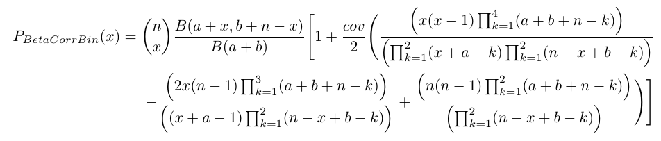
x = 0,1,2,3,...n

n = 1,2,3,...

0 < a,b

-\infty < cov < +\infty

0 < p < 1

p=\frac{a}{a+b}

\Theta=\frac{1}{a+b}

The Correlation is in between

\frac{-2}{n(n-1)} min(\frac{p}{1-p},\frac{1-p}{p}) \le correlation \le \frac{2p(1-p)}{(n-1)p(1-p)+0.25-fo}

where fo=min [(x-(n-1)p-0.5)^2]

The mean and the variance are denoted as

E_{BetaCorrBin}[x]= np

Var_{BetaCorrBin}[x]= np(1-p)(n\Theta+1)(1+\Theta)^{-1}+n(n-1)cov

Corr_{BetaCorrBin}[x]=\frac{cov}{p(1-p)}

NOTE : If input parameters are not in given domain conditions necessary error messages will be provided to go further.

Value

The output of dBetaCorrBin gives a list format consisting

pdf probability function values in vector form.

mean mean of Beta-Correlated Binomial Distribution.

var variance of Beta-Correlated Binomial Distribution.

corr correlation of Beta-Correlated Binomial Distribution.

mincorr minimum correlation value possible.

maxcorr maximum correlation value possible.

References

Paul SR (1985). “A three-parameter generalization of the binomial distribution.” History and Philosophy of Logic, 14(6), 1497–1506.

Examples

#plotting the random variables and probability values
col <- rainbow(5)
a <- c(9.0,10,11,12,13)
b <- c(8.0,8.1,8.2,8.3,8.4)
plot(0,0,main="Beta-Correlated binomial probability function graph",xlab="Binomial random variable",
ylab="Probability function values",xlim = c(0,10),ylim = c(0,0.5))
for (i in 1:5)
{
lines(0:10,dBetaCorrBin(0:10,10,0.001,a[i],b[i])$pdf,col = col[i],lwd=2.85)
points(0:10,dBetaCorrBin(0:10,10,0.001,a[i],b[i])$pdf,col = col[i],pch=16)
}

dBetaCorrBin(0:10,10,0.001,10,13)$pdf      #extracting the pdf values
dBetaCorrBin(0:10,10,0.001,10,13)$mean     #extracting the mean
dBetaCorrBin(0:10,10,0.001,10,13)$var      #extracting the variance
dBetaCorrBin(0:10,10,0.001,10,13)$corr     #extracting the correlation
dBetaCorrBin(0:10,10,0.001,10,13)$mincorr  #extracting the minimum correlation value
dBetaCorrBin(0:10,10,0.001,10,13)$maxcorr  #extracting the maximum correlation value

#plotting the random variables and cumulative probability values
col <- rainbow(5)
a <- c(9.0,10,11,12,13)
b <- c(8.0,8.1,8.2,8.3,8.4)
plot(0,0,main="Beta-Correlated binomial probability function graph",xlab="Binomial random variable",
ylab="Probability function values",xlim = c(0,10),ylim = c(0,1))
for (i in 1:5)
{
lines(0:10,pBetaCorrBin(0:10,10,0.001,a[i],b[i]),col = col[i],lwd=2.85)
points(0:10,pBetaCorrBin(0:10,10,0.001,a[i],b[i]),col = col[i],pch=16)
}

pBetaCorrBin(0:10,10,0.001,10,13)      #acquiring the cumulative probability values

COM Poisson Binomial Distribution

Description

These functions provide the ability for generating probability function values and cumulative probability function values for the COM Poisson Binomial Distribution.

Usage

dCOMPBin(x,n,p,v)

Arguments

x

vector of binomial random variables.

n

single value for no of binomial trials.

p

single value for probability of success.

v

single value for v.

Details

The probability function and cumulative function can be constructed and are denoted below

The cumulative probability function is the summation of probability function values.

P_{COMPBin}(x) = \frac{{n \choose x}^v p^x (1-p)^{n-x}}{\sum_{j=0}^{n} {n \choose j}^v p^j (1-p)^{(n-j)}}

x = 0,1,2,3,...n

n = 1,2,3,...

0 < p < 1

-\infty < v < +\infty

NOTE : If input parameters are not in given domain conditions necessary error messages will be provided to go further.

Value

The output of dCOMPBin gives a list format consisting

pdf probability function values in vector form.

mean mean of COM Poisson Binomial Distribution.

var variance of COM Poisson Binomial Distribution.

References

Examples

#plotting the random variables and probability values
col <- rainbow(5)
a <- c(0.58,0.59,0.6,0.61,0.62)
b <- c(0.022,0.023,0.024,0.025,0.026)
plot(0,0,main="COM Poisson Binomial probability function graph",xlab="Binomial random variable",
ylab="Probability function values",xlim = c(0,10),ylim = c(0,0.5))
for (i in 1:5)
{
lines(0:10,dCOMPBin(0:10,10,a[i],b[i])$pdf,col = col[i],lwd=2.85)
points(0:10,dCOMPBin(0:10,10,a[i],b[i])$pdf,col = col[i],pch=16)
}

dCOMPBin(0:10,10,0.58,0.022)$pdf      #extracting the pdf values
dCOMPBin(0:10,10,0.58,0.022)$mean     #extracting the mean
dCOMPBin(0:10,10,0.58,0.022)$var      #extracting the variance

#plotting the random variables and cumulative probability values
col <- rainbow(5)
a <- c(0.58,0.59,0.6,0.61,0.62)
b <- c(0.022,0.023,0.024,0.025,0.026)
plot(0,0,main="COM Poisson Binomial probability function graph",xlab="Binomial random variable",
ylab="Probability function values",xlim = c(0,10),ylim = c(0,1))
for (i in 1:5)
{
lines(0:10,pCOMPBin(0:10,10,a[i],b[i]),col = col[i],lwd=2.85)
points(0:10,pCOMPBin(0:10,10,a[i],b[i]),col = col[i],pch=16)
}

pCOMPBin(0:10,10,0.58,0.022)      #acquiring the cumulative probability values

Correlated Binomial Distribution

Description

These functions provide the ability for generating probability function values and cumulative probability function values for the Correlated Binomial Distribution.

Usage

dCorrBin(x,n,p,cov)

Arguments

x

vector of binomial random variables.

n

single value for no of binomial trials.

p

single value for probability of success.

cov

single value for covariance.

Details

The probability function and cumulative function can be constructed and are denoted below

The cumulative probability function is the summation of probability function values.

P_{CorrBin}(x) = {n \choose x}(p^x)(1-p)^{n-x}(1+(\frac{cov}{2p^2(1-p)^2})((x-np)^2+x(2p-1)-np^2))

x = 0,1,2,3,...n

n = 1,2,3,...

0 < p < 1

-\infty < cov < +\infty

The Correlation is in between

\frac{-2}{n(n-1)} min(\frac{p}{1-p},\frac{1-p}{p}) \le correlation \le \frac{2p(1-p)}{(n-1)p(1-p)+0.25-fo}

where fo=min [(x-(n-1)p-0.5)^2]

The mean and the variance are denoted as

E_{CorrBin}[x]= np

Var_{CorrBin}[x]= n(p(1-p)+(n-1)cov)

Corr_{CorrBin}[x]=\frac{cov}{p(1-p)}

NOTE : If input parameters are not in given domain conditions necessary error messages will be provided to go further.

Value

The output of dCorrBin gives a list format consisting

pdf probability function values in vector form.

mean mean of Correlated Binomial Distribution.

var variance of Correlated Binomial Distribution.

corr correlation of Correlated Binomial Distribution.

mincorr minimum correlation value possible.

maxcorr maximum correlation value possible.

References

Examples

#plotting the random variables and probability values
col <- rainbow(5)
a <- c(0.58,0.59,0.6,0.61,0.62)
b <- c(0.022,0.023,0.024,0.025,0.026)
plot(0,0,main="Correlated binomial probability function graph",xlab="Binomial random variable",
ylab="Probability function values",xlim = c(0,10),ylim = c(0,0.5))
for (i in 1:5)
{
lines(0:10,dCorrBin(0:10,10,a[i],b[i])$pdf,col = col[i],lwd=2.85)
points(0:10,dCorrBin(0:10,10,a[i],b[i])$pdf,col = col[i],pch=16)
}

dCorrBin(0:10,10,0.58,0.022)$pdf      #extracting the pdf values
dCorrBin(0:10,10,0.58,0.022)$mean     #extracting the mean
dCorrBin(0:10,10,0.58,0.022)$var      #extracting the variance
dCorrBin(0:10,10,0.58,0.022)$corr     #extracting the correlation
dCorrBin(0:10,10,0.58,0.022)$mincorr  #extracting the minimum correlation value
dCorrBin(0:10,10,0.58,0.022)$maxcorr  #extracting the maximum correlation value

#plotting the random variables and cumulative probability values
col <- rainbow(5)
a <- c(0.58,0.59,0.6,0.61,0.62)
b <- c(0.022,0.023,0.024,0.025,0.026)
plot(0,0,main="Correlated binomial probability function graph",xlab="Binomial random variable",
ylab="Probability function values",xlim = c(0,10),ylim = c(0,1))
for (i in 1:5)
{
lines(0:10,pCorrBin(0:10,10,a[i],b[i]),col = col[i],lwd=2.85)
points(0:10,pCorrBin(0:10,10,a[i],b[i]),col = col[i],pch=16)
}

pCorrBin(0:10,10,0.58,0.022)      #acquiring the cumulative probability values

Gamma Distribution

Description

These functions provide the ability for generating probability density values, cumulative probability density values and moment about zero values for Gamma Distribution bounded between [0,1].

Usage

dGAMMA(p,c,l)

Arguments

p

vector of probabilities.

c

single value for shape parameter c.

l

single value for shape parameter l.

Details

The probability density function and cumulative density function of a unit bounded Gamma distribution with random variable P are given by

g_{P}(p) = \frac{ c^l p^{c-1}}{\gamma(l)} [ln(1/p)]^{l-1}

; 0 \le p \le 1

G_{P}(p) = \frac{ Ig(l,cln(1/p))}{\gamma(l)}

; 0 \le p \le 1

l,c > 0

The mean the variance are denoted by

E[P] = (\frac{c}{c+1})^l

var[P] = (\frac{c}{c+2})^l - (\frac{c}{c+1})^{2l}

The moments about zero is denoted as

E[P^r]=(\frac{c}{c+r})^l

r = 1,2,3,...

Defined as \gamma(l) is the gamma function Defined as Ig(l,cln(1/p))= \int_0^{cln(1/p)} t^{l-1} e^{-t}dt is the Lower incomplete gamma function

NOTE : If input parameters are not in given domain conditions necessary error messages will be provided to go further.

Value

The output of dGAMMA gives a list format consisting

pdf probability density values in vector form.

mean mean of the Gamma distribution.

var variance of Gamma distribution.

References

Olshen AC (1938). “Transformations of the pearson type III distribution.” The Annals of Mathematical Statistics, 9(3), 176–200.

Examples

#plotting the random variables and probability values
col <- rainbow(4)
a <- c(1,2,5,10)
plot(0,0,main="Probability density graph",xlab="Random variable",ylab="Probability density values",
xlim = c(0,1),ylim = c(0,4))
for (i in 1:4)
{
lines(seq(0,1,by=0.01),dGAMMA(seq(0,1,by=0.01),a[i],a[i])$pdf,col = col[i])
}

dGAMMA(seq(0,1,by=0.01),5,6)$pdf   #extracting the pdf values
dGAMMA(seq(0,1,by=0.01),5,6)$mean  #extracting the mean
dGAMMA(seq(0,1,by=0.01),5,6)$var   #extracting the variance

#plotting the random variables and cumulative probability values
col <- rainbow(4)
a <- c(1,2,5,10)
plot(0,0,main="Cumulative density graph",xlab="Random variable",ylab="Cumulative density values",
xlim = c(0,1),ylim = c(0,1))
for (i in 1:4)
{
lines(seq(0,1,by=0.01),pGAMMA(seq(0,1,by=0.01),a[i],a[i]),col = col[i])
}

pGAMMA(seq(0,1,by=0.01),5,6)   #acquiring the cumulative probability values
mazGAMMA(1.4,5,6)              #acquiring the moment about zero values
mazGAMMA(2,5,6)-mazGAMMA(1,5,6)^2 #acquiring the variance for a=5,b=6

#only the integer value of moments is taken here because moments cannot be decimal
mazGAMMA(1.9,5.5,6)

Generalized Beta Type-1 Distribution

Description

These functions provide the ability for generating probability density values, cumulative probability density values and moment about zero values for the Generalized Beta Type-1 Distribution bounded between [0,1].

Usage

dGBeta1(p,a,b,c)

Arguments

p

vector of probabilities.

a

single value for shape parameter alpha representing as a.

b

single value for shape parameter beta representing as b.

c

single value for shape parameter gamma representing as c.

Details

The probability density function and cumulative density function of a unit bounded Generalized Beta Type-1 Distribution with random variable P are given by

g_{P}(p)= \frac{c}{B(a,b)} p^{ac-1} (1-p^c)^{b-1}

; 0 \le p \le 1

G_{P}(p)= \frac{p^{ac}}{aB(a,b)} 2F1(a,1-b;p^c;a+1)

0 \le p \le 1

a,b,c > 0

The mean and the variance are denoted by

E[P]= \frac{B(a+b,\frac{1}{c})}{B(a,\frac{1}{c})}

var[P]= \frac{B(a+b,\frac{2}{c})}{B(a,\frac{2}{c})}-(\frac{B(a+b,\frac{1}{c})}{B(a,\frac{1}{c})})^2

The moments about zero is denoted as

E[P^r]= \frac{B(a+b,\frac{r}{c})}{B(a,\frac{r}{c})}

r = 1,2,3,....

Defined as B(a,b) is Beta function. Defined as 2F1(a,b;c;d) is Gaussian Hypergeometric function.

NOTE : If input parameters are not in given domain conditions necessary error messages will be provided to go further.

Value

The output of dGBeta1 gives a list format consisting

pdf probability density values in vector form.

mean mean of the Generalized Beta Type-1 Distribution.

var variance of the Generalized Beta Type-1 Distribution.

References

Examples

#plotting the random variables and probability values
col <- rainbow(5)
a <- c(.1,.2,.3,1.5,2.15)
plot(0,0,main="Probability density graph",xlab="Random variable",ylab="Probability density values",
xlim = c(0,1),ylim = c(0,10))
for (i in 1:5)
{
lines(seq(0,1,by=0.001),dGBeta1(seq(0,1,by=0.001),a[i],1,2*a[i])$pdf,col = col[i])
}

dGBeta1(seq(0,1,by=0.01),2,3,1)$pdf    #extracting the pdf values
dGBeta1(seq(0,1,by=0.01),2,3,1)$mean   #extracting the mean
dGBeta1(seq(0,1,by=0.01),2,3,1)$var    #extracting the variance

pGBeta1(0.04,2,3,4)        #acquiring the cdf values for a=2,b=3,c=4
mazGBeta1(1.4,3,2,2)              #acquiring the moment about zero values
mazGBeta1(2,3,2,2)-mazGBeta1(1,3,2,2)^2        #acquiring the variance for a=3,b=2,c=2

#only the integer value of moments is taken here because moments cannot be decimal
mazGBeta1(3.2,3,2,2)

Gaussian Hypergeometric Generalized Beta Binomial Distribution

Description

These functions provide the ability for generating probability function values and cumulative probability function values for the Gaussian Hypergeometric Generalized Beta Binomial distribution.

Usage

dGHGBB(x,n,a,b,c)

Arguments

x

vector of binomial random variables.

n

single value for no of binomial trials.

a

single value for shape parameter alpha value representing a.

b

single value for shape parameter beta value representing b.

c

single value for shape parameter lambda value representing c.

Details

Mixing Gaussian Hypergeometric Generalized Beta distribution with Binomial distribution will create the Gaussian Hypergeometric Generalized Beta Binomial distribution. The probability function and cumulative probability function can be constructed and are denoted below.

The cumulative probability function is the summation of probability function values.

P_{GHGBB}(x)=\frac{1}{2F1(-n,a;-b-n+1;c)} {n \choose x} \frac{B(x+a,n-x+b)}{B(a,b+n)}(c^x)

a,b,c > 0

x = 0,1,2,...n

n = 1,2,3,...

The mean, variance and over dispersion are denoted as

E_{GHGBB}[x]= nE_{GHGBeta}

Var_{GHGBB}[x]= nE_{GHGBeta}(1-E_{GHGBeta})+ n(n-1)Var_{GHGBeta}

over dispersion= \frac{var_{GHGBeta}}{E_{GHGBeta}(1-E_{GHGBeta})}

Defined as B(a,b) is the beta function. Defined as 2F1(a,b;c;d) is the Gaussian Hypergeometric function

NOTE : If input parameters are not in given domain conditions necessary error messages will be provided to go further.

Value

The output of dGHGBB gives a list format consisting

pdf probability function values in vector form.

mean mean of Gaussian Hypergeometric Generalized Beta Binomial Distribution.

var variance of Gaussian Hypergeometric Generalized Beta Binomial Distribution.

over.dis.para over dispersion value of Gaussian Hypergeometric Generalized Beta Binomial Distribution.

References

Examples

#plotting the random variables and probability values
col <- rainbow(6)
a <- c(.1,.2,.3,1.5,2.1,3)
plot(0,0,main="GHGBB probability function graph",xlab="Binomial random variable",
ylab="Probability function values",xlim = c(0,7),ylim = c(0,0.9))
for (i in 1:6)
{
lines(0:7,dGHGBB(0:7,7,1+a[i],0.3,1+a[i])$pdf,col = col[i],lwd=2.85)
points(0:7,dGHGBB(0:7,7,1+a[i],0.3,1+a[i])$pdf,col = col[i],pch=16)
}

dGHGBB(0:7,7,1.3,0.3,1.3)$pdf      #extracting the pdf values
dGHGBB(0:7,7,1.3,0.3,1.3)$mean     #extracting the mean
dGHGBB(0:7,7,1.3,0.3,1.3)$var      #extracting the variance
dGHGBB(0:7,7,1.3,0.3,1.3)$over.dis.par  #extracting the over dispersion value

#plotting the random variables and cumulative probability values
col <- rainbow(4)
a <- c(1,2,5,10)
plot(0,0,main="Cumulative probability function graph",xlab="Binomial random variable",
ylab="Cumulative probability function values",xlim = c(0,7),ylim = c(0,1))
for (i in 1:4)
{
lines(0:7,pGHGBB(0:7,7,1+a[i],0.3,1+a[i]),col = col[i])
points(0:7,pGHGBB(0:7,7,1+a[i],0.3,1+a[i]),col = col[i])
}

pGHGBB(0:7,7,1.3,0.3,1.3)     #acquiring the cumulative probability values

Gaussian Hypergeometric Generalized Beta Distribution

Description

These functions provide the ability for generating probability density values, cumulative probability density values and moment about zero values for the Gaussian Hypergeometric Generalized Beta distribution bounded between [0,1].

Usage

dGHGBeta(p,n,a,b,c)

Arguments

p

vector of probabilities.

n

single value for no of binomial trials.

a

single value for shape parameter alpha representing as a.

b

single value for shape parameter beta representing as b.

c

single value for shape parameter lambda representing as c.

Details

The probability density function and cumulative density function of a unit bounded Gaussian Hypergeometric Generalized Beta Distribution with random variable P are given by

g_{P}(p)= \frac{1}{B(a,b)}\frac{2F1(-n,a;-b-n+1;1)}{2F1(-n,a;-b-n+1;c)} p^{a-1}(1-p)^{b-1} \frac{c^{b+n}}{(c+(1-c)p)^{a+b+n}}

; 0 \le p \le 1

G_{P}(p)= \int^p_0 \frac{1}{B(a,b)}\frac{2F1(-n,a;-b-n+1;1)}{2F1(-n,a;-b-n+1;c)} t^{a-1}(1-t)^{b-1}\frac{c^{b+n}}{(c+(1-c)t)^{a+b+n}} \,dt

; 0 \le p \le 1

a,b,c > 0

n = 1,2,3,...

The mean and the variance are denoted by

E[P]= \int^1_0 \frac{p}{B(a,b)}\frac{2F1(-n,a;-b-n+1;1)}{2F1(-n,a;-b-n+1;c)} p^{a-1}(1-p)^{b-1}\frac{c^{b+n}}{(c+(1-c)p)^{a+b+n}} \,dp

var[P]= \int^1_0 \frac{p^2}{B(a,b)}\frac{2F1(-n,a;-b-n+1;1)}{2F1(-n,a;-b-n+1;c)} p^{a-1}(1-p)^{b-1}\frac{c^{b+n}}{(c+(1-c)p)^{a+b+n}} \,dp - (E[p])^2

The moments about zero is denoted as

E[P^r]= \int^1_0 \frac{p^r}{B(a,b)}\frac{2F1(-n,a;-b-n+1;1)}{2F1(-n,a;-b-n+1;c)} p^{a-1}(1-p)^{b-1}\frac{c^{b+n}}{(c+(1-c)p)^{a+b+n}} \,dp

r = 1,2,3,...

Defined as B(a,b) as the beta function. Defined as 2F1(a,b;c;d) as the Gaussian Hypergeometric function.

NOTE : If input parameters are not in given domain conditions necessary error messages will be provided to go further.

Value

The output of dGHGBeta gives a list format consisting

pdf probability density values in vector form.

mean mean of the Gaussian Hypergeometric Generalized Beta Distribution.

var variance of the Gaussian Hypergeometric Generalized Beta Distribution.

References

Examples

#plotting the random variables and probability values
col <- rainbow(5)
a <- c(.1,.2,.3,1.5,2.15)
plot(0,0,main="Probability density graph",xlab="Random variable",ylab="Probability density values",
xlim = c(0,1),ylim = c(0,10))
for (i in 1:5)
{
lines(seq(0,1,by=0.001),dGHGBeta(seq(0,1,by=0.001),7,1+a[i],0.3,1+a[i])$pdf,col = col[i])
}

dGHGBeta(seq(0,1,by=0.01),7,1.6312,0.3913,0.6659)$pdf   #extracting the pdf values
dGHGBeta(seq(0,1,by=0.01),7,1.6312,0.3913,0.6659)$mean  #extracting the mean
dGHGBeta(seq(0,1,by=0.01),7,1.6312,0.3913,0.6659)$var   #extracting the variance

#plotting the random variables and cumulative probability values
col <- rainbow(6)
a <- c(.1,.2,.3,1.5,2.1,3)
plot(0,0,main="Cumulative density graph",xlab="Random variable",ylab="Cumulative density values",
xlim = c(0,1),ylim = c(0,1))
for (i in 1:6)
{
lines(seq(0.01,1,by=0.001),pGHGBeta(seq(0.01,1,by=0.001),7,1+a[i],0.3,1+a[i]),col=col[i])
}

pGHGBeta(seq(0,1,by=0.01),7,1.6312,0.3913,0.6659) #acquiring the cumulative probability values
mazGHGBeta(1.4,7,1.6312,0.3913,0.6659)            #acquiring the moment about zero values

#acquiring the variance for a=1.6312,b=0.3913,c=0.6659
mazGHGBeta(2,7,1.6312,0.3913,0.6659)-mazGHGBeta(1,7,1.6312,0.3913,0.6659)^2

#only the integer value of moments is taken here because moments cannot be decimal
mazGHGBeta(1.9,15,5,6,1)

Gamma Binomial Distribution

Description

These functions provide the ability for generating probability function values and cumulative probability function values for the Gamma Binomial Distribution.

Usage

dGammaBin(x,n,c,l)

Arguments

x

vector of binomial random variables.

n

single value for no of binomial trials.

c

single value for shape parameter c.

l

single value for shape parameter l.

Details

Mixing Gamma distribution with Binomial distribution will create the the Gamma Binomial distribution. The probability function and cumulative probability function can be constructed and are denoted below.

The cumulative probability function is the summation of probability function values.

P_{GammaBin}[x]= {n \choose x} \sum_{j=0}^{n-x} {n-x \choose j} (-1)^j (\frac{c}{c+x+j})^l

c,l > 0

x = 0,1,2,...,n

n = 1,2,3,...

The mean, variance and over dispersion are denoted as

E_{GammaBin}[x] = (\frac{c}{c+1})^l

Var_{GammaBin}[x] = n^2[(\frac{c}{c+2})^l - (\frac{c}{c+1})^{2l}] + n(\frac{c}{c+1})^l{1-)(\frac{c+1}{c+2})^l}

over dispersion= \frac{(\frac{c}{c+2})^l - (\frac{c}{c+1})^{2l}}{(\frac{c}{c+1})^l[1-(\frac{c}{c+1})^l]}

Value

The output of dGammaBin gives a list format consisting

pdf probability function values in vector form.

mean mean of the Gamma Binomial Distribution.

var variance of the Gamma Binomial Distribution.

over.dis.para over dispersion value of the Gamma Binomial Distribution.

References

Examples

#plotting the random variables and probability values
col <- rainbow(5)
a <- c(1,2,5,10,0.2)
plot(0,0,main="Gamma Binomial probability function graph",xlab="Binomial random variable",
ylab="Probability function values",xlim = c(0,10),ylim = c(0,0.5))
for (i in 1:5)
{
lines(0:10,dGammaBin(0:10,10,a[i],a[i])$pdf,col = col[i],lwd=2.85)
points(0:10,dGammaBin(0:10,10,a[i],a[i])$pdf,col = col[i],pch=16)
}

dGammaBin(0:10,10,4,.2)$pdf    #extracting the pdf values
dGammaBin(0:10,10,4,.2)$mean   #extracting the mean
dGammaBin(0:10,10,4,.2)$var    #extracting the variance
dGammaBin(0:10,10,4,.2)$over.dis.para  #extracting the over dispersion value

#plotting the random variables and cumulative probability values
col <- rainbow(4)
a <- c(1,2,5,10)
plot(0,0,main="Cumulative probability function graph",xlab="Binomial random variable",
ylab="Cumulative probability function values",xlim = c(0,10),ylim = c(0,1))
for (i in 1:4)
{
lines(0:10,pGammaBin(0:10,10,a[i],a[i]),col = col[i])
points(0:10,pGammaBin(0:10,10,a[i],a[i]),col = col[i])
}

pGammaBin(0:10,10,4,.2)   #acquiring the cumulative probability values

Grassia-II-Binomial Distribution

Description

These functions provide the ability for generating probability function values and cumulative probability function values for the Grassia-II-Binomial Distribution.

Usage

dGrassiaIIBin(x,n,a,b)

Arguments

x

vector of binomial random variables.

n

single value for no of binomial trials.

a

single value for shape parameter a.

b

single value for shape parameter b.

Details

Mixing Gamma distribution with Binomial distribution will create the the Grassia-II-Binomial distribution, only when (1-p)=e^(-lambda) of the Binomial distribution. The probability function and cumulative probability function can be constructed and are denoted below.

The cumulative probability function is the summation of probability function values.

P_{GrassiaIIBin}[x]= {n \choose x} \sum_{j=0}^{x} {x \choose j} (-1)^{x-j} (1+b(n-j))^{-a}

a,b > 0

x = 0,1,2,...,n

n = 1,2,3,...

The mean, variance and over dispersion are denoted as

E_{GrassiaIIBin}[x] = (\frac{b}{b+1})^a

Var_{GrassiaIIBin}[x] = n^2[(\frac{b}{b+2})^a - (\frac{b}{b+1})^{2a}] + n(\frac{b}{b+1})^a{1-(\frac{b+1}{b+2})^a}

over dispersion= \frac{(\frac{b}{b+2})^l - (\frac{b}{b+1})^{2a}}{(\frac{b}{b+1})^a[1-(\frac{b}{b+1})^a]}

Value

The output of dGrassiaIIBin gives a list format consisting

pdf probability function values in vector form.

mean mean of the Grassia II Binomial Distribution.

var variance of the Grassia II Binomial Distribution.

over.dis.para over dispersion value of the Grassia II Binomial Distribution.

References

Examples

#plotting the random variables and probability values
col <- rainbow(5)
a <- c(1,2,5,10,0.2)
plot(0,0,main="Grassia II binomial probability function graph",xlab="Binomial random variable",
ylab="Probability function values",xlim = c(0,10),ylim = c(0,0.5))
for (i in 1:5)
{
lines(0:10,dGrassiaIIBin(0:10,10,a[i],a[i])$pdf,col = col[i],lwd=2.85)
points(0:10,dGrassiaIIBin(0:10,10,a[i],a[i])$pdf,col = col[i],pch=16)
}

dGrassiaIIBin(0:10,10,4,.2)$pdf    #extracting the pdf values
dGrassiaIIBin(0:10,10,4,.2)$mean   #extracting the mean
dGrassiaIIBin(0:10,10,4,.2)$var    #extracting the variance
dGrassiaIIBin(0:10,10,4,.2)$over.dis.para  #extracting the over dispersion value

#plotting the random variables and cumulative probability values
col <- rainbow(4)
a <-c (1,2,5,10)
plot(0,0,main="Cumulative probability function graph",xlab="Binomial random variable",
ylab="Cumulative probability function values",xlim = c(0,10),ylim = c(0,1))
for (i in 1:4)
{
lines(0:10,pGrassiaIIBin(0:10,10,a[i],a[i]),col = col[i])
points(0:10,pGrassiaIIBin(0:10,10,a[i],a[i]),col = col[i])
}

pGrassiaIIBin(0:10,10,4,.2)   #acquiring the cumulative probability values

Kumaraswamy Distribution

Description

These functions provide the ability for generating probability density values, cumulative probability density values and moment about zero values for the Kumaraswamy Distribution bounded between [0,1].

Usage

dKUM(p,a,b)

Arguments

p

vector of probabilities.

a

single value for shape parameter alpha representing as a.

b

single value for shape parameter beta representing as b.

Details

The probability density function and cumulative density function of a unit bounded Kumaraswamy Distribution with random variable P are given by

g_{P}(p)= abp^{a-1}(1-p^a)^{b-1}

; 0 \le p \le 1

G_{P}(p)= 1-(1-p^a)^b

; 0 \le p \le 1

a,b > 0

The mean and the variance are denoted by

E[P]= bB(1+\frac{1}{a},b)

var[P]= bB(1+\frac{2}{a},b)-(bB(1+\frac{1}{a},b))^2

The moments about zero is denoted as

E[P^r]= bB(1+\frac{r}{a},b)

r = 1,2,3,...

Defined as B(a,b) is the beta function.

NOTE : If input parameters are not in given domain conditions necessary error messages will be provided to go further.

Value

The output of dKUM gives a list format consisting

pdf probability density values in vector form.

mean mean of the Kumaraswamy distribution.

var variance of the Kumaraswamy distribution.

References

Kumaraswamy P (1980). “A generalized probability density function for double-bounded random processes.” Journal of hydrology, 46(1-2), 79–88. Jones MC (2009). “Kumaraswamy’s distribution: A beta-type distribution with some tractability advantages.” Statistical methodology, 6(1), 70–81.

Examples

#plotting the random variables and probability values
col <- rainbow(4)
a <- c(1,2,5,10)
plot(0,0,main="Probability density graph",xlab="Random variable",ylab="Probability density values",
xlim = c(0,1),ylim = c(0,6))
for (i in 1:4)
{
lines(seq(0,1,by=0.01),dKUM(seq(0,1,by=0.01),a[i],a[i])$pdf,col = col[i])
}

dKUM(seq(0,1,by=0.01),2,3)$pdf   #extracting the probability values
dKUM(seq(0,1,by=0.01),2,3)$mean  #extracting the mean
dKUM(seq(0,1,by=0.01),2,3)$var   #extracting the variance

#plotting the random variables and cumulative probability values
col <- rainbow(4)
a <- c(1,2,5,10)
plot(0,0,main="Cumulative density graph",xlab="Random variable",ylab="Cumulative density values",
xlim = c(0,1),ylim = c(0,1))
for (i in 1:4)
{
lines(seq(0,1,by=0.01),pKUM(seq(0,1,by=0.01),a[i],a[i]),col = col[i])
}

pKUM(seq(0,1,by=0.01),2,3)    #acquiring the cumulative probability values

mazKUM(1.4,3,2)               #acquiring the moment about zero values
mazKUM(2,2,3)-mazKUM(1,2,3)^2  #acquiring the variance for a=2,b=3

#only the integer value of moments is taken here because moments cannot be decimal
mazKUM(1.9,5.5,6)

Kumaraswamy Binomial Distribution

Description

These functions provide the ability for generating probability function values and cumulative probability function values for the Kumaraswamy Binomial Distribution.

Usage

dKumBin(x,n,a,b,it=25000)

Arguments

x

vector of binomial random variables

n

single value for no of binomial trial

a

single value for shape parameter alpha representing a

b

single value for shape parameter beta representing b

it

number of iterations to converge as a proper probability function replacing infinity

Details

Mixing Kumaraswamy distribution with Binomial distribution will create the Kumaraswamy Binomial distribution. The probability function and cumulative probability function can be constructed and are denoted below.

The cumulative probability function is the summation of probability function values.

P_{KumBin}(x)= ab{n \choose x} \sum_{j=0}^{it} (-1)^j{b-1 \choose j}B(x+a+aj,n-x+1)

a,b > 0

x = 0,1,2,...n

n = 1,2,3,...

it > 0

The mean, variance and over dispersion are denoted as

E_{KumBin}[x]= nbB(1+\frac{1}{a},b)

Var_{KumBin}[x]= n^2 b(B(1+\frac{2}{a},b)-bB(1+\frac{1}{a},b)^2)+ nb(B(1+\frac{1}{a},b)-B(1+\frac{2}{a},b))

over dispersion= \frac{(bB(1+\frac{2}{a},b)-(bB(1+\frac{1}{a},b))^2)} {(bB(1+\frac{1}{a},b)-(bB(1+\frac{1}{a},b))^2)}

Defined as B(a,b) is the beta function.

NOTE : If input parameters are not in given domain conditions necessary error messages will be provided to go further.

Value

The output of dKumBin gives a list format consisting

pdf probability function values in vector form.

mean mean of the Kumaraswamy Binomial Distribution.

var variance of the Kumaraswamy Binomial Distribution.

over.dis.para over dispersion value of the Kumaraswamy Distribution.

References

Xiaohu L, Yanyan H, Xueyan Z (2011). “The Kumaraswamy binomial distribution.” Chinese Journal of Applied Probability and Statistics, 27(5), 511–521.

Examples

## Not run: 
#plotting the random variables and probability values
col <- rainbow(5)
a <- c(1,2,5,10,.85)
plot(0,0,main="Kumaraswamy binomial probability function graph",xlab="Binomial random variable",
ylab="Probability function values",xlim = c(0,10),ylim = c(0,0.5))
for (i in 1:5) {
lines(0:10,dKumBin(0:10,10,a[i],a[i])$pdf,col = col[i],lwd=2.85)
points(0:10,dKumBin(0:10,10,a[i],a[i])$pdf,col = col[i],pch=16)
  }

## End(Not run)

dKumBin(0:10,10,4,2)$pdf  #extracting the pdf values
dKumBin(0:10,10,4,2)$mean #extracting the mean
dKumBin(0:10,10,4,2)$var  #extracting the variance
dKumBin(0:10,10,4,2)$over.dis.para #extracting the over dispersion value

## Not run: 
#plotting the random variables and cumulative probability values
col <- rainbow(5)
a <- c(1,2,5,10,.85)
plot(0,0,main="Cumulative probability function graph",xlab="Binomial random variable",
ylab="Cumulative probability function values",xlim = c(0,10),ylim = c(0,1))
for (i in 1:5) {
lines(0:10,pKumBin(0:10,10,a[i],a[i]),col = col[i])
points(0:10,pKumBin(0:10,10,a[i],a[i]),col = col[i])
  }

## End(Not run)

pKumBin(0:10,10,4,2)    #acquiring the cumulative probability values

Lovinson Multiplicative Binomial Distribution

Description

These functions provide the ability for generating probability function values and cumulative probability function values for the Lovinson Multiplicative Binomial Distribution.

Usage

dLMBin(x,n,p,phi)

Arguments

x

vector of binomial random variables.

n

single value for no of binomial trials.

p

single value for probability of success.

phi

single value for phi.

Details

The probability function and cumulative function can be constructed and are denoted below

The cumulative probability function is the summation of probability function values.

P_{LMBin}(x)= {n \choose x} p^x (1-p)^{n-x} \frac{(phi^{x(n-x)}}{f(p,phi,n)}

here f(p,phi,n) is

f(p,phi,n)= \sum_{k=0}^{n} {n \choose k} p^k (1-p)^{n-k} (phi^{k(n-k)} )

x = 0,1,2,3,...n

n = 1,2,3,...

k = 0,1,2,...,n

0 < p < 1

0 < phi

NOTE : If input parameters are not in given domain conditions necessary error messages will be provided to go further.

Value

The output of dLMBin gives a list format consisting

pdf probability function values in vector form.

mean mean of Lovinson Multiplicative Binomial Distribution.

var variance of Lovinson Multiplicative Binomial Distribution.

References

Examples

#plotting the random variables and probability values
col <- rainbow(5)
a <- c(0.58,0.59,0.6,0.61,0.62)
b <- c(0.022,0.023,0.024,0.025,0.026)
plot(0,0,main="Lovinson Multiplicative binomial probability
     function graph",xlab="Binomial random variable",
     ylab="Probability function values",xlim = c(0,10),ylim = c(0,0.5))
for (i in 1:5)
{
lines(0:10,dLMBin(0:10,10,a[i],1+b[i])$pdf,col = col[i],lwd=2.85)
points(0:10,dLMBin(0:10,10,a[i],1+b[i])$pdf,col = col[i],pch=16)
}

dLMBin(0:10,10,.58,10.022)$pdf   #extracting the pdf values
dLMBin(0:10,10,.58,10.022)$mean   #extracting the mean
dLMBin(0:10,10,.58,10.022)$var   #extracting the variance


#plotting random variables and cumulative probability values
col <- rainbow(5)
a <- c(0.58,0.59,0.6,0.61,0.62)
b <- c(0.022,0.023,0.024,0.025,0.026)
plot(0,0,main="Lovinson Multiplicative binomial probability
     function graph",xlab="Binomial random variable",
     ylab="Probability function values",xlim = c(0,10),ylim = c(0,1))
for (i in 1:5)
{
lines(0:10,pLMBin(0:10,10,a[i],1+b[i]),col = col[i],lwd=2.85)
points(0:10,pLMBin(0:10,10,a[i],1+b[i]),col = col[i],pch=16)
}

pLMBin(0:10,10,.58,10.022)     #acquiring the cumulative probability values

McDonald Generalized Beta Binomial Distribution

Description

These functions provide the ability for generating probability function values and cumulative probability function values for the McDonald Generalized Beta Binomial Distribution.

Usage

dMcGBB(x,n,a,b,c)

Arguments

x

vector of binomial random variables.

n

single value for no of binomial trials.

a

single value for shape parameter alpha representing as a.

b

single value for shape parameter beta representing as b.

c

single value for shape parameter gamma representing as c.

Details

Mixing Generalized Beta Type-1 Distribution with Binomial distribution the probability function value and cumulative probability function can be constructed and are denoted below.

The cumulative probability function is the summation of probability function values.

P_{McGBB}(x)= {n \choose x} \frac{1}{B(a,b)} (\sum_{j=0}^{n-x} (-1)^j {n-x \choose j} B(\frac{x}{c}+a+\frac{j}{c},b) )

a,b,c > 0

The mean, variance and over dispersion are denoted as

E_{McGBB}[x]= n\frac{B(a+b,\frac{1}{c})}{B(a,\frac{1}{c})}

Var_{McGBB}[x]= n^2(\frac{B(a+b,\frac{2}{c})}{B(a,\frac{2}{c})}-(\frac{B(a+b,\frac{1}{c})}{B(a,\frac{1}{c})})^2) +n(\frac{B(a+b,\frac{1}{c})}{B(a,\frac{1}{c})}-\frac{B(a+b,\frac{2}{c})}{B(a,\frac{2}{c})})

over dispersion= \frac{\frac{B(a+b,\frac{2}{c})}{B(a,\frac{2}{c})}-(\frac{B(a+b,\frac{1}{c})}{B(a,\frac{1}{c})})^2}{\frac{B(a+b,\frac{1}{c})}{B(a,\frac{1}{c})}-(\frac{B(a+b,\frac{1}{c})}{B(a,\frac{1}{c})})^2}

x = 0,1,2,...n

n = 1,2,3,...

Value

The output of dMcGBB gives a list format consisting

pdf probability function values in vector form.

mean mean of McDonald Generalized Beta Binomial Distribution.

var variance of McDonald Generalized Beta Binomial Distribution.

over.dis.para over dispersion value of McDonald Generalized Beta Binomial Distribution.

References

Examples

#plotting the random variables and probability values
col <- rainbow(5)
a <- c(1,2,5,10,0.6)
plot(0,0,main="Mcdonald generalized beta-binomial probability function graph",
xlab="Binomial random variable",ylab="Probability function values",xlim = c(0,10),ylim = c(0,0.5))
for (i in 1:5)
{
lines(0:10,dMcGBB(0:10,10,a[i],2.5,a[i])$pdf,col = col[i],lwd=2.85)
points(0:10,dMcGBB(0:10,10,a[i],2.5,a[i])$pdf,col = col[i],pch=16)
}

dMcGBB(0:10,10,4,2,1)$pdf             #extracting the pdf values
dMcGBB(0:10,10,4,2,1)$mean            #extracting the mean
dMcGBB(0:10,10,4,2,1)$var             #extracting the variance
dMcGBB(0:10,10,4,2,1)$over.dis.para   #extracting the over dispersion value

#plotting the random variables and cumulative probability values
col <- rainbow(4)
a <- c(1,2,5,10)
plot(0,0,main="Cumulative probability function graph",xlab="Binomial random variable",
ylab="Cumulative probability function values",xlim = c(0,10),ylim = c(0,1))
for (i in 1:4)
{
lines(0:10,pMcGBB(0:10,10,a[i],a[i],2),col = col[i])
points(0:10,pMcGBB(0:10,10,a[i],a[i],2),col = col[i])
}

pMcGBB(0:10,10,4,2,1)       #acquiring the cumulative probability values

Multiplicative Binomial Distribution

Description

These functions provide the ability for generating probability function values and cumulative probability function values for the Multiplicative Binomial Distribution.

Usage

dMultiBin(x,n,p,theta)

Arguments

x

vector of binomial random variables.

n

single value for no of binomial trials.

p

single value for probability of success.

theta

single value for theta.

Details

The probability function and cumulative function can be constructed and are denoted below

The cumulative probability function is the summation of probability function values.

P_{MultiBin}(x)= {n \choose x} p^x (1-p)^{n-x} \frac{(theta^{x(n-x)}}{f(p,theta,n)}

here f(p,theta,n) is

f(p,theta,n)= \sum_{k=0}^{n} {n \choose k} p^k (1-p)^{n-k} (theta^{k(n-k)} )

x = 0,1,2,3,...n

n = 1,2,3,...

k = 0,1,2,...,n

0 < p < 1

0 < theta

NOTE : If input parameters are not in given domain conditions necessary error messages will be provided to go further.

Value

The output of dMultiBin gives a list format consisting

pdf probability function values in vector form.

mean mean of Multiplicative Binomial Distribution.

var variance of Multiplicative Binomial Distribution.

References

Examples

#plotting the random variables and probability values
col <- rainbow(5)
a <- c(0.58,0.59,0.6,0.61,0.62)
b <- c(0.022,0.023,0.024,0.025,0.026)
plot(0,0,main="Multiplicative binomial probability function graph",xlab="Binomial random variable",
ylab="Probability function values",xlim = c(0,10),ylim = c(0,0.5))
for (i in 1:5)
{
lines(0:10,dMultiBin(0:10,10,a[i],1+b[i])$pdf,col = col[i],lwd=2.85)
points(0:10,dMultiBin(0:10,10,a[i],1+b[i])$pdf,col = col[i],pch=16)
}

dMultiBin(0:10,10,.58,10.022)$pdf   #extracting the pdf values
dMultiBin(0:10,10,.58,10.022)$mean   #extracting the mean
dMultiBin(0:10,10,.58,10.022)$var   #extracting the variance


#plotting random variables and cumulative probability values
col <- rainbow(5)
a <- c(0.58,0.59,0.6,0.61,0.62)
b <- c(0.022,0.023,0.024,0.025,0.026)
plot(0,0,main="Multiplicative binomial probability function graph",xlab="Binomial random variable",
ylab="Probability function values",xlim = c(0,10),ylim = c(0,1))
for (i in 1:5)
{
lines(0:10,pMultiBin(0:10,10,a[i],1+b[i]),col = col[i],lwd=2.85)
points(0:10,pMultiBin(0:10,10,a[i],1+b[i]),col = col[i],pch=16)
}

pMultiBin(0:10,10,.58,10.022)     #acquiring the cumulative probability values

Triangular Distribution Bounded Between [0,1]

Description

These functions provide the ability for generating probability density values, cumulative probability density values and moments about zero values for the Triangular Distribution bounded between [0,1].

Usage

dTRI(p,mode)

Arguments

p

vector of probabilities.

mode

single value for mode.

Details

Setting min=0 and max=1 mode=c in the Triangular distribution a unit bounded Triangular distribution can be obtained. The probability density function and cumulative density function of a unit bounded Triangular distribution with random variable P are given by

g_{P}(p)= \frac{2p}{c}

; 0 \le p < c

g_{P}(p)= \frac{2(1-p)}{(1-c)}

; c \le p \le 1

G_{P}(p)= \frac{p^2}{c}

; 0 \le p < c

G_{P}(p)= 1-\frac{(1-p)^2}{(1-c)}

; c \le p \le 1

0 \le mode=c \le 1

The mean and the variance are denoted by

E[P]= \frac{(a+b+c)}{3}= \frac{(1+c)}{3}

var[P]= \frac{a^2+b^2+c^2-ab-ac-bc}{18}= \frac{(1+c^2-c)}{18}

Moments about zero is denoted as

E[P^r]= \frac{2c^{r+2}}{c(r+2)}+\frac{2(1-c^{r+1})}{(1-c)(r+1)}+\frac{2(c^{r+2}-1)}{(1-c)(r+2)}

r = 1,2,3,...

NOTE : If input parameters are not in given domain conditions necessary error messages will be provided to go further.

Value

The output of dTRI gives a list format consisting

pdf probability density values in vector form.

mean mean of the unit bounded Triangular distribution.

variance variance of the unit bounded Triangular distribution

References

Horsnell G (1957). “Economical acceptance sampling schemes.” Journal of the Royal Statistical Society. Series A (General), 120(2), 148–201. Johnson NL, Kotz S, Balakrishnan N (1995). Continuous univariate distributions, volume 2, volume 289. John wiley and sons. Karlis D, Xekalaki E (2008). The polygonal distribution. Springer. Okagbue HI, Edeki SO, Opanuga AA, Oguntunde PE, Adeosun ME (2014). “Using the Average of the Extreme Values of a Triangular Distribution for a Transformation, and Its Approximant via the Continuous Uniform Distribution.” British Journal of Mathematics and Computer Science, 4(24), 3497.

Examples

#plotting the random variables and probability values
col <- rainbow(4)
x <- seq(0.2,0.8,by=0.2)
plot(0,0,main="Probability density graph",xlab="Random variable",
ylab="Probability density values",xlim = c(0,1),ylim = c(0,3))
for (i in 1:4)
{
lines(seq(0,1,by=0.01),dTRI(seq(0,1,by=0.01),x[i])$pdf,col = col[i])
}

dTRI(seq(0,1,by=0.05),0.3)$pdf     #extracting the pdf values
dTRI(seq(0,1,by=0.01),0.3)$mean    #extracting the mean
dTRI(seq(0,1,by=0.01),0.3)$var     #extracting the variance

#plotting the random variables and cumulative probability values
col <- rainbow(4)
x <- seq(0.2,0.8,by=0.2)
plot(0,0,main="Cumulative density graph",xlab="Random variable",
ylab="Cumulative density values",xlim = c(0,1),ylim = c(0,1))
for (i in 1:4)
{
lines(seq(0,1,by=0.01),pTRI(seq(0,1,by=0.01),x[i]),col = col[i])
}

pTRI(seq(0,1,by=0.05),0.3)      #acquiring the cumulative probability values
mazTRI(1.4,.3)                  #acquiring the moment about zero values
mazTRI(2,.3)-mazTRI(1,.3)^2     #variance for when is mode 0.3

#only the integer value of moments is taken here because moments cannot be decimal
mazTRI(1.9,0.5)

Triangular Binomial Distribution

Description

These functions provide the ability for generating probability function values and cumulative probability function values for the Triangular Binomial distribution.

Usage

dTriBin(x,n,mode)

Arguments

x

vector of binomial random variables.

n

single value for no of binomial trials.

mode

single value for mode.

Details

Mixing unit bounded Triangular distribution with Binomial distribution will create Triangular Binomial distribution. The probability function and cumulative probability function can be constructed and are denoted below.

The cumulative probability function is the summation of probability function values.

P_{TriBin}(x)= 2 {n \choose x}(c^{-1}B_c(x+2,n-x+1)+(1-c)^{-1}B(x+1,n-x+2)-(1-c)^{-1}B_c(x+1,n-x+2))

0 < mode=c < 1

x = 0,1,2,...n

n = 1,2,3...

The mean, variance and over dispersion are denoted as

E_{TriiBin}[x]= \frac{n(1+c)}{3}

Var_{TriBin}[x]= \frac{n(n+3)}{18}-\frac{n(n-3)c(1-c)}{18}

over dispersion= \frac{(1-c+c^2)}{2(2+c-c^2)}

Defined as B_c(a,b)=\int^c_0 t^{a-1} (1-t)^{b-1} \,dt is incomplete beta integrals and B(a,b) is the beta function.

NOTE : If input parameters are not in given domain conditions necessary error messages will be provided to go further.

Value

The output of dTriBin gives a list format consisting

pdf probability function values in vector form.

mean mean of the Triangular Binomial Distribution.

var variance of the Triangular Binomial Distribution.

over.dis.para over dispersion value of the Triangular Binomial Distribution.

References

Examples

#plotting the random variables and probability values
col <- rainbow(7)
x <- seq(0.1,0.7,by=0.1)
plot(0,0,main="Triangular binomial probability function graph",xlab="Binomial random variable",
ylab="Probability function values",xlim = c(0,10),ylim = c(0,.3))
for (i in 1:7)
{
lines(0:10,dTriBin(0:10,10,x[i])$pdf,col = col[i],lwd=2.85)
points(0:10,dTriBin(0:10,10,x[i])$pdf,col = col[i],pch=16)
}

dTriBin(0:10,10,.4)$pdf        #extracting the pdf values
dTriBin(0:10,10,.4)$mean       #extracting the mean
dTriBin(0:10,10,.4)$var        #extracting the variance
dTriBin(0:10,10,.4)$over.dis.para  #extracting the over dispersion value

#plotting the random variables and cumulative probability values
col <- rainbow(7)
x <- seq(0.1,0.7,by=0.1)
plot(0,0,main="Triangular binomial probability function graph",xlab="Binomial random variable",
ylab="Probability function values",xlim = c(0,10),ylim = c(0,1))
for (i in 1:7)
{
lines(0:10,pTriBin(0:10,10,x[i]),col = col[i],lwd=2.85)
points(0:10,pTriBin(0:10,10,x[i]),col = col[i],pch=16)
}

pTriBin(0:10,10,.4)    #acquiring the cumulative probability values

Uniform Distribution Bounded Between [0,1]

Description

These functions provide the ability for generating probability density values, cumulative probability density values and moments about zero values for the Uniform Distribution bounded between [0,1].

Usage

dUNI(p)

Arguments

p

vector of probabilities.

Details

Setting a=0 and b=1 in the Uniform Distribution a unit bounded Uniform Distribution can be obtained. The probability density function and cumulative density function of a unit bounded Uniform Distribution with random variable P are given by

g_{P}(p) = 1

0 \le p \le 1

G_{P}(p) = p

0 \le p \le 1

The mean and the variance are denoted as

E[P]= \frac{1}{a+b}= 0.5

var[P]= \frac{(b-a)^2}{12}= 0.0833

Moments about zero is denoted as

E[P^r]= \frac{e^{rb}-e^{ra}}{r(b-a)}= \frac{e^r-1}{r}

r = 1,2,3,...

NOTE : If input parameters are not in given domain conditions necessary error messages will be provided to go further.

Value

The output of dUNI gives a list format consisting

pdf probability density values in vector form.

mean mean of unit bounded uniform distribution.

var variance of unit bounded uniform distribution.

References

Examples

#plotting the random variables and probability values
plot(seq(0,1,by=0.01),dUNI(seq(0,1,by=0.01))$pdf,type = "l",main="Probability density graph",
xlab="Random variable",ylab="Probability density values")

dUNI(seq(0,1,by=0.05))$pdf     #extract the pdf values
dUNI(seq(0,1,by=0.01))$mean    #extract the mean
dUNI(seq(0,1,by=0.01))$var     #extract the variance

#plotting the random variables and cumulative probability values
plot(seq(0,1,by=0.01),pUNI(seq(0,1,by=0.01)),type = "l",main="Cumulative density graph",
xlab="Random variable",ylab="Cumulative density values")

pUNI(seq(0,1,by=0.05))     #acquiring the cumulative probability values

mazUNI(c(1,2,3))    #acquiring the moment about zero values

#only the integer value of moments is taken here because moments cannot be decimal
mazUNI(1.9)

Uniform Binomial Distribution

Description

These functions provide the ability for generating probability function values and cumulative probability function values for the Uniform Binomial Distribution.

Usage

dUniBin(x,n)

Arguments

x

vector of binomial random variables.

n

single value for no of binomial trials.

Details

Mixing unit bounded uniform distribution with binomial distribution will create the Uniform Binomial Distribution. The probability function and cumulative probability function can be constructed and are denoted below.

The cumulative probability function is the summation of probability function values

P_{UniBin}(x)= \frac{1}{n+1}

n = 1,2,...

x = 0,1,2,...n

The mean, variance and over dispersion are denoted as

E_{UniBin}[X]= \frac{n}{2}

Var_{UniBin}[X]= \frac{n(n+2)}{12}

over dispersion= \frac{1}{3}

NOTE : If input parameters are not in given domain conditions necessary error messages will be provided to go further.

Value

The output of dUniBin gives a list format consisting

pdf probability function values in vector form.

mean mean of the Uniform Binomial Distribution.

var variance of the Uniform Binomial Distribution.

ove.dis.para over dispersion value of Uniform Binomial Distribution.

References

Horsnell G (1957). “Economical acceptance sampling schemes.” Journal of the Royal Statistical Society. Series A (General), 120(2), 148–201. Okagbue HI, Edeki SO, Opanuga AA, Oguntunde PE, Adeosun ME (2014). “Using the Average of the Extreme Values of a Triangular Distribution for a Transformation, and Its Approximant via the Continuous Uniform Distribution.” British Journal of Mathematics and Computer Science, 4(24), 3497.

Examples

#plotting the binomial random variables and probability values
plot(0:10,dUniBin(0:10,10)$pdf,type="l",main="Uniform binomial probability function graph",
xlab=" Binomial random variable",ylab="Probability function values")
points(0:10,dUniBin(0:10,10)$pdf)

dUniBin(0:300,300)$pdf  #extracting the pdf values
dUniBin(0:10,10)$mean   #extracting the mean
dUniBin(0:10,10)$var    #extracting the variance
dUniBin(0:10,10)$over.dis.para  #extracting the over dispersion

#plotting the binomial random variables and cumulative probability values
plot(0:10,pUniBin(0:10,10),type="l",main="Cumulative probability function graph",
xlab=" Binomial random variable",ylab="Cumulative probability function values")
points(0:10,pUniBin(0:10,10))

pUniBin(0:15,15)       #acquiring the cumulative probability values

Fitting the Additive Binomial Distribution when binomial random variable, frequency, probability of success and alpha are given

Description

The function will fit the Additive Binomial distribution when random variables, corresponding frequencies, probability of success and alpha are given. It will provide the expected frequencies, chi-squared test statistics value, p value, and degree of freedom value so that it can be seen if this distribution fits the data.

Usage

fitAddBin(x,obs.freq,p,alpha)

Arguments

x

vector of binomial random variables.

obs.freq

vector of frequencies.

p

single value for probability of success.

alpha

single value for alpha.

Details

obs.freq \ge 0

x = 0,1,2,..

0 < p < 1

-1 < alpha < 1

Value

The output of fitAddBin gives the class format fitAB and fit consisting a list

bin.ran.var binomial random variables.

obs.freq corresponding observed frequencies.

exp.freq corresponding expected frequencies.

statistic chi-squared test statistics.

df degree of freedom.

p.value probability value by chi-squared test statistic.

fitAB fitted probability values of dAddBin.

NegLL Negative Log Likelihood value.

p estimated probability value.

alpha estimated alpha parameter value.

AIC AIC value.

call the inputs of the function.

Methods summary, print, AIC, residuals and fitted can be used to extract specific outputs.

References

Examples

No.D.D <- 0:7         #assigning the random variables
Obs.fre.1 <- c(47,54,43,40,40,41,39,95)            #assigning the corresponding the frequencies

## Not run: 
#assigning the estimated probability value
paddbin <- EstMLEAddBin(No.D.D,Obs.fre.1)$p

#assigning the estimated alpha value
alphaaddbin <- EstMLEAddBin(No.D.D,Obs.fre.1)$alpha

#fitting when the random variable,frequencies,probability and alpha are given
results <- fitAddBin(No.D.D,Obs.fre.1,paddbin,alphaaddbin)
results

#extracting the AIC value
AIC(results)

#extract fitted values
fitted(results)

## End(Not run)

Fitting the Beta-Binomial Distribution when binomial random variable, frequency and shape parameters a and b are given

Description

The function will fit the Beta-Binomial distribution when random variables, corresponding frequencies and shape parameters are given. It will provide the expected frequencies, chi-squared test statistics value, p value, degree of freedom and over dispersion value so that it can be seen if this distribution fits the data.

Usage

fitBetaBin(x,obs.freq,a,b)

Arguments

x

vector of binomial random variables.

obs.freq

vector of frequencies.

a

single value for shape parameter alpha representing as a.

b

single value for shape parameter beta representing as b.

Details

0 < a,b

x = 0,1,2,...,n

obs.freq \ge 0

NOTE : If input parameters are not in given domain conditions necessary error messages will be provided to go further.

Value

The output of fitBetaBin gives the class format fitBB and fit consisting a list

bin.ran.var binomial random variables.

obs.freq corresponding observed frequencies.

exp.freq corresponding expected frequencies.

statistic chi-squared test statistics.

df degree of freedom.

p.value probability value by chi-squared test statistic.

fitBB fitted values of dBetaBin.

NegLL Negative Log Likelihood value.

a estimated value for alpha parameter as a.

b estimated value for alpha parameter as b.

AIC AIC value.

over.dis.para over dispersion value.

call the inputs of the function.

Methods summary, print, AIC, residuals and fitted can be used to extract specific outputs.

References

Examples

No.D.D <- 0:7    #assigning the random variables
Obs.fre.1 <- c(47,54,43,40,40,41,39,95)  #assigning the corresponding frequencies

#estimating the parameters using maximum log likelihood value and assigning it
parameters <- EstMLEBetaBin(No.D.D,Obs.fre.1,0.1,0.1)

bbmle::coef(parameters)   #extracting the parameters a and b
aBetaBin <- bbmle::coef(parameters)[1]  #assigning the parameter a
bBetaBin <- bbmle::coef(parameters)[2]  #assigning the parameter b

#fitting when the random variable,frequencies,shape parameter values are given.
fitBetaBin(No.D.D,Obs.fre.1,aBetaBin,bBetaBin)

#estimating the parameters using moment generating function methods
results <- EstMGFBetaBin(No.D.D,Obs.fre.1)
results

aBetaBin1 <- results$a  #assigning the estimated a
bBetaBin1 <- results$b  #assigning the estimated b

#fitting when the random variable,frequencies,shape parameter values are given.
BB <- fitBetaBin(No.D.D,Obs.fre.1,aBetaBin1,bBetaBin1)

#extracting the expected frequencies
fitted(BB)

#extracting the residuals
residuals(BB)

Fitting the Beta-Correlated Binomial Distribution when binomial random variable, frequency, covariance, alpha and beta parameters are given

Description

The function will fit the Beta-Correlated Binomial Distribution when random variables, corresponding frequencies, covariance, alpha and beta parameters are given. It will provide the expected frequencies, chi-squared test statistics value, p value, and degree of freedom so that it can be seen if this distribution fits the data.

Usage

fitBetaCorrBin(x,obs.freq,cov,a,b)

Arguments

x

vector of binomial random variables.

obs.freq

vector of frequencies.

cov

single value for covariance.

a

single value for alpha parameter.

b

single value for beta parameter.

Details

obs.freq \ge 0

x = 0,1,2,..

-\infty < cov < +\infty

0 < a,b

NOTE : If input parameters are not in given domain conditions necessary error messages will be provided to go further.

Value

The output of fitBetaCorrBin gives the class format fitBCB and fit consisting a list

bin.ran.var binomial random variables.

obs.freq corresponding observed frequencies.

exp.freq corresponding expected frequencies.

statistic chi-squared test statistics.

df degree of freedom.

p.value probability value by chi-squared test statistic

corr Correlation value.

fitBCB fitted probability values of dBetaCorrBin.

NegLL Negative Log Likelihood value.

a estimated shape parameter value a.

b estimated shape parameter value b.

cov estimated covariance value.

AIC AIC value.

call the inputs of the function.

Methods summary, print, AIC, residuals and fitted can be used to extract specific outputs.

References

Paul SR (1985). “A three-parameter generalization of the binomial distribution.” History and Philosophy of Logic, 14(6), 1497–1506.

Examples

No.D.D <- 0:7                    #assigning the random variables
Obs.fre.1 <- c(47,54,43,40,40,41,39,95)      #assigning the corresponding frequencies

#estimating the parameters using maximum log likelihood value and assigning it
parameters <- EstMLEBetaCorrBin(x=No.D.D,freq=Obs.fre.1,cov=0.0050,a=10,b=10)

covBetaCorrBin <- bbmle::coef(parameters)[1]
aBetaCorrBin <- bbmle::coef(parameters)[2]
bBetaCorrBin <- bbmle::coef(parameters)[3]

#fitting when the random variable,frequencies,covariance, a and b are given
results <- fitBetaCorrBin(No.D.D,Obs.fre.1,covBetaCorrBin,aBetaCorrBin,bBetaCorrBin)
results

#extract AIC value
AIC(results)

#extract fitted values
fitted(results)

Fitting the Binomial Distribution when binomial random variable, frequency and probability value are given

Description

The function will fit the Binomial distribution when random variables, corresponding frequencies and probability value are given. It will provide the expected frequencies, chi-squared test statistics value, p value and degree of freedom so that it can be seen if this distribution fits the data.

Usage

fitBin(x,obs.freq,p=0)

Arguments

x

vector of binomial random variables.

obs.freq

vector of frequencies.

p

single value for probability or zero to estimate p.

Details

x = 0,1,2,...

0 < p <= 1

obs.freq \ge 0

NOTE : If input parameters are not in given domain conditions necessary error messages will be provided to go further.

Value

The output of fitBin gives the class format fitB and fit consisting a list

bin.ran.var binomial random variables.

obs.freq corresponding observed frequencies.

exp.freq corresponding expected frequencies.

statistic chi-squared test statistics value.

df degree of freedom.

p.value probability value by chi-squared test statistic.

fitB fitted probability values of dbinom.

phat estimated probability value.

call the inputs of the function.

Examples

No.D.D <- 0:7      #assigning the random variables
Obs.fre.1 <- c(47,54,43,40,40,41,39,95)  #assigning the corresponding frequencies

#fitting when the random variable,frequencies are given.
fitBin(No.D.D,Obs.fre.1)

Fitting the COM Poisson Binomial Distribution when binomial random variable, frequency, probability of success and v parameter are given

Description

The function will fit the COM Poisson Binomial Distribution when random variables, corresponding frequencies, probability of success and v parameter are given. It will provide the expected frequencies, chi-squared test statistics value, p value, and degree of freedom so that it can be seen if this distribution fits the data.

Usage

fitCOMPBin(x,obs.freq,p,v)

Arguments

x

vector of binomial random variables.

obs.freq

vector of frequencies.

p

single value for probability of success.

v

single value for v.

Details

obs.freq \ge 0

x = 0,1,2,..

0 < p < 1

-\infty < v < +\infty

NOTE : If input parameters are not in given domain conditions necessary error messages will be provided to go further.

Value

The output of fitCOMPBin gives the class format fitCPB and fit consisting a list

bin.ran.var binomial random variables.

obs.freq corresponding observed frequencies.

exp.freq corresponding expected frequencies.

statistic chi-squared test statistics.

df degree of freedom.

p.value probability value by chi-squared test statistic.

fitCPB fitted probability values of dCOMPBin.

NegLL Negative Log Likelihood value.

p estimated probability value.

v estimated v parameter value.

AIC AIC value.

call the inputs of the function.

Methods summary, print, AIC, residuals and fitted can be used to extract specific outputs.

References

Examples

No.D.D <- 0:7                    #assigning the random variables
Obs.fre.1 <- c(47,54,43,40,40,41,39,95)      #assigning the corresponding frequencies

#estimating the parameters using maximum log likelihood value and assigning it
parameters <- EstMLECOMPBin(x=No.D.D,freq=Obs.fre.1,p=0.5,v=0.050)

pCOMPBin <- bbmle::coef(parameters)[1]
vCOMPBin <- bbmle::coef(parameters)[2]

#fitting when the random variable,frequencies,probability and v parameter are given
results <- fitCOMPBin(No.D.D,Obs.fre.1,pCOMPBin,vCOMPBin)
results

#extracting the AIC value
AIC(results)

#extract fitted values
fitted(results)

Fitting the Correlated Binomial Distribution when binomial random variable, frequency, probability of success and covariance are given

Description

The function will fit the Correlated Binomial Distribution when random variables, corresponding frequencies, probability of success and covariance are given. It will provide the expected frequencies, chi-squared test statistics value, p value, and degree of freedom so that it can be seen if this distribution fits the data.

Usage

fitCorrBin(x,obs.freq,p,cov)

Arguments

x

vector of binomial random variables.

obs.freq

vector of frequencies.

p

single value for probability of success.

cov

single value for covariance.

Details

obs.freq \ge 0

x = 0,1,2,..

0 < p < 1

-\infty < cov < +\infty

NOTE : If input parameters are not in given domain conditions necessary error messages will be provided to go further.

Value

The output of fitCorrBin gives the class format fitCB and fit consisting a list

bin.ran.var binomial random variables.

obs.freq corresponding observed frequencies.

exp.freq corresponding expected frequencies.

statistic chi-squared test statistics.

df degree of freedom.

p.value probability value by chi-squared test statistic.

corr Correlation value.

fitCB fitted probability values of dCorrBin.

NegLL Negative Log Likelihood value.

AIC AIC value.

call the inputs of the function.

Methods summary, print, AIC, residuals and fitted can be used to extract specific outputs.

References

Examples

No.D.D <- 0:7       #assigning the random variables
Obs.fre.1 <- c(47,54,43,40,40,41,39,95)      #assigning the corresponding frequencies

#estimating the parameters using maximum log likelihood value and assigning it
parameters <- EstMLECorrBin(x=No.D.D,freq=Obs.fre.1,p=0.5,cov=0.0050)

pCorrBin <- bbmle::coef(parameters)[1]
covCorrBin <- bbmle::coef(parameters)[2]

#fitting when the random variable,frequencies,probability and covariance are given
results <- fitCorrBin(No.D.D,Obs.fre.1,pCorrBin,covCorrBin)
results

#extracting the AIC value
AIC(results)

#extract fitted values
fitted(results)

Fitting the Gaussian Hypergeometric Generalized Beta Binomial Distribution when binomial random variable, frequency and shape parameters a,b and c are given

Description

The function will fit the Gaussian Hypergeometric Generalized Beta Binomial Distribution when random variables, corresponding frequencies and shape parameters are given. It will provide the expected frequencies, chi-squared test statistics value, p value, degree of freedom and over dispersion value so that it can be seen if this distribution fits the data.

Usage

fitGHGBB(x,obs.freq,a,b,c)

Arguments

x

vector of binomial random variables.

obs.freq

vector of frequencies.

a

single value for shape parameter alpha representing a.

b

single value for shape parameter beta representing b.

c

single value for shape parameter lambda representing c.

Details

0 < a,b,c

x = 0,1,2,...

obs.freq \ge 0

NOTE : If input parameters are not in given domain conditions necessary error messages will be provided to go further.

Value

The output of fitGHGBB gives the class format fitGB and fit consisting a list

bin.ran.var binomial random variables.

obs.freq corresponding observed frequencies.

exp.freq corresponding expected frequencies.

statistic chi-squared test statistics.

df degree of freedom.

p.value probability value by chi-squared test statistic.

fitGB fitted values of dGHGBB.

NegLL Negative Loglikelihood value.

a estimated value for alpha parameter as a.

b estimated value for beta parameter as b.

c estimated value for gamma parameter as c.

AIC AIC value.

over.dis.para over dispersion value.

call the inputs of the function.

Methods summary, print, AIC, residuals and fitted can be used to extract specific outputs.

References

Examples

No.D.D <- 0:7        #assigning the random variables
Obs.fre.1 <- c(47,54,43,40,40,41,39,95)       #assigning the corresponding frequencies

#estimating the parameters using maximum log likelihood value and assigning it
parameters <- EstMLEGHGBB(No.D.D,Obs.fre.1,0.1,20,1.3)

bbmle::coef(parameters)         #extracting the parameters
aGHGBB <- bbmle::coef(parameters)[1]  #assigning the estimated a
bGHGBB <- bbmle::coef(parameters)[2]  #assigning the estimated b
cGHGBB <- bbmle::coef(parameters)[3]  #assigning the estimated c

#fitting when the random variable,frequencies,shape parameter values are given.
results <- fitGHGBB(No.D.D,Obs.fre.1,aGHGBB,bGHGBB,cGHGBB)
results

#extracting the expected frequencies
fitted(results)

#extracting the residuals
residuals(results)

Fitting the Gamma Binomial distribution when binomial random variable, frequency and shape parameters are given

Description

The function will fit the Gamma Binomial Distribution when random variables, corresponding frequencies and shape parameters are given. It will provide the expected frequencies, chi-squared test statistics value, p value, degree of freedom and over dispersion value so that it can be seen if this distribution fits the data.

Usage

fitGammaBin(x,obs.freq,c,l)

Arguments

x

vector of binomial random variables.

obs.freq

vector of frequencies.

c

single value for shape parameter c.

l

single value for shape parameter l.

Details

0 < c,l

x = 0,1,2,...

obs.freq \ge 0

NOTE : If input parameters are not in given domain conditions necessary error messages will be provided to go further.

Value

The output of fitGammaBin gives the class format fitGaB and fit consisting a list

bin.ran.var binomial random variables.

obs.freq corresponding observed frequencies.

exp.freq corresponding expected frequencies.

statistic chi-squared test statistics.

df degree of freedom.

p.value probability value by chi-squared test statistic.

fitMB fitted values of dGammaBin.

NegLL Negative Log Likelihood value.

c estimated value for shape parameter c.

l estimated value for shape parameter l.

AIC AIC value.

over.dis.para over dispersion value.

call the inputs of the function.

Methods summary, print, AIC, residuals and fitted can be used to extract specific outputs.

References

Examples

No.D.D <- 0:7       #assigning the random variables
Obs.fre.1 <- c(47,54,43,40,40,41,39,95)          #assigning the corresponding frequencies

#estimating the parameters using maximum log likelihood value and assigning it
parameters <- EstMLEGammaBin(x=No.D.D,freq=Obs.fre.1,c=0.1,l=0.1)

cGBin <- bbmle::coef(parameters)[1]         #assigning the estimated c
lGBin <- bbmle::coef(parameters)[2]         #assigning the estimated l

#fitting when the random variable,frequencies,shape parameter values are given.
results <- fitGammaBin(No.D.D,Obs.fre.1,cGBin,lGBin)
results

#extracting the expected frequencies
fitted(results)

#extracting the residuals
residuals(results)

Fitting the Grassia II Binomial distribution when binomial random variable, frequency and shape parameters are given

Description

The function will fit the Grassia II Binomial Distribution when random variables, corresponding frequencies and shape parameters are given. It will provide the expected frequencies, chi-squared test statistics value, p value, degree of freedom and over dispersion value so that it can be seen if this distribution fits the data.

Usage

fitGrassiaIIBin(x,obs.freq,a,b)

Arguments

x

vector of binomial random variables.

obs.freq

vector of frequencies.

a

single value for shape parameter a.

b

single value for shape parameter b.

Details

0 < a,b

x = 0,1,2,...

obs.freq \ge 0

NOTE : If input parameters are not in given domain conditions necessary error messages will be provided to go further.

Value

The output of fitGrassiaIIBin gives the class format fitGrIIB and fit consisting a list

bin.ran.var binomial random variables.

obs.freq corresponding observed frequencies.

exp.freq corresponding expected frequencies.

statistic chi-squared test statistics.

df degree of freedom.

p.value probability value by chi-squared test statistic.

fitGrIIB fitted values of dGrassiaIIBin.

NegLL Negative Log Likelihood value.

a estimated value for shape parameter a.

b estimated value for shape parameter b.

AIC AIC value.

over.dis.para over dispersion value.

call the inputs of the function.

Methods summary, print, AIC, residuals and fitted can be used to extract specific outputs.

References

Examples

No.D.D <- 0:7       #assigning the random variables
Obs.fre.1 <- c(47,54,43,40,40,41,39,95)          #assigning the corresponding frequencies

#estimating the parameters using maximum log likelihood value and assigning it
parameters <- EstMLEGrassiaIIBin(x=No.D.D,freq=Obs.fre.1,a=0.1,b=0.1)

aGIIBin <- bbmle::coef(parameters)[1]         #assigning the estimated a
bGIIBin <- bbmle::coef(parameters)[2]         #assigning the estimated b

#fitting when the random variable,frequencies,shape parameter values are given.
results <- fitGrassiaIIBin(No.D.D,Obs.fre.1,aGIIBin,bGIIBin)
results

#extracting the expected frequencies
fitted(results)

#extracting the residuals
residuals(results)

Fitting the Kumaraswamy Binomial Distribution when binomial random variable, frequency and shape parameters a and b, iterations parameter it are given

Description

The function will fit the Kumaraswamy Binomial distribution when random variables, corresponding frequencies and shape parameters are given. It will provide the expected frequencies, chi-squared test statistics value, p value, degree of freedom and over dispersion value so that it can be seen if this distribution fits the data.

Usage

fitKumBin(x,obs.freq,a,b,it)

Arguments

x

vector of binomial random variables.

obs.freq

vector of frequencies.

a

single value for shape parameter alpha representing a.

b

single value for shape parameter beta representing b.

it

number of iterations to converge as a proper probability function replacing infinity.

Details

0 < a,b

x = 0,1,2,...n

obs.freq \ge 0

it > 0

NOTE : If input parameters are not in given domain conditions necessary error messages will be provided to go further.

Value

The output of fitKumBin gives the class format fitKB and fit consisting a list

bin.ran.var binomial random variables.

obs.freq corresponding observed frequencies.

exp.freq corresponding expected frequencies.

statistic chi-squared test statistics.

df degree of freedom.

p.value probability value by chi-squared test statistic.

fitKB fitted values of dKumBin.

NegLL Negative Log Likelihood value.

a estimated value for alpha parameter as a.

b estimated value for beta parameter as b.

it estimated it value for iterations.

AIC AIC value.

over.dis.para over dispersion value.

call the inputs of the function.

Methods summary, print, AIC, residuals and fiited can be used to extract specific outputs.

References

Xiaohu L, Yanyan H, Xueyan Z (2011). “The Kumaraswamy binomial distribution.” Chinese Journal of Applied Probability and Statistics, 27(5), 511–521.

Examples

No.D.D <- 0:7   #assigning the random variables
Obs.fre.1 <- c(47,54,43,40,40,41,39,95)   #assigning the corresponding frequencies

## Not run: 
#estimating the parameters using maximum log likelihood value and assigning it
parameters <- EstMLEKumBin(x=No.D.D,freq=Obs.fre.1,a=10.1,b=1.1,it=10000)

bbmle::coef(parameters)    #extracting the parameters
aKumBin <- bbmle::coef(parameters)[1] #assigning the estimated a
bKumBin <- bbmle::coef(parameters)[2] #assigning the estimated b
itKumBin <- bbmle::coef(parameters)[3] #assigning the estimated iterations

#fitting when the random variable,frequencies,shape parameter values are given.
results <- fitKumBin(No.D.D,Obs.fre.1,aKumBin,bKumBin,itKumBin*100)
results

#extracting the expected frequencies
fitted(results)

#extracting the residuals
residuals(results)

## End(Not run)

Fitting the Lovinson Multiplicative Binomial Distribution when binomial random variable, frequency, probability of success and theta parameter are given

Description

The function will fit the Lovinson Multiplicative Binomial distribution when random variables, corresponding frequencies, probability of success and phi parameter are given. It will provide the expected frequencies, chi-squared test statistics value, p value and degree of freedom value so that it can be seen if this distribution fits the data.

Usage

fitLMBin(x,obs.freq,p,phi)

Arguments

x

vector of binomial random variables.

obs.freq

vector of frequencies.

p

single value for probability of success.

phi

single value for phi parameter.

Details

obs.freq \ge 0

x = 0,1,2,..

0 < p < 1

0 < phi

Value

The output of fitLMBin gives the class format fitLMB and fit consisting a list

bin.ran.var binomial random variables.

obs.freq corresponding observed frequencies.

exp.freq corresponding expected frequencies.

statistic chi-squared test statistics.

df degree of freedom.

p.value probability value by chi-squared test statistic.

fitLMB fitted probability values of dLMBin.

NegLL Negative Log Likelihood value.

p estimated probability value.

phi estimated phi parameter value.

AIC AIC value.

call the inputs of the function.

Methods summary, print, AIC, residuals and fitted can be used to extract specific outputs.

References

Examples

No.D.D <- 0:7       #assigning the random variables
Obs.fre.1 <- c(47,54,43,40,40,41,39,95)     #assigning the corresponding frequencies

#estimating the parameters using maximum log likelihood value and assigning it
parameters <- EstMLELMBin(x=No.D.D,freq=Obs.fre.1,p=0.1,phi=.3)

pLMBin=bbmle::coef(parameters)[1]    #assigning the estimated probability value
phiLMBin <- bbmle::coef(parameters)[2]  #assigning the estimated phi value

#fitting when the random variable,frequencies,probability and phi are given
results <- fitLMBin(No.D.D,Obs.fre.1,pLMBin,phiLMBin)
results

#extracting the AIC value
AIC(results)

#extract fitted values
fitted(results)

Fitting the McDonald Generalized Beta Binomial distribution when binomial random variable, frequency and shape parameters are given

Description

The function will fit the McDonald Generalized Beta Binomial Distribution when random variables, corresponding frequencies and shape parameters are given. It will provide the expected frequencies, chi-squared test statistics value, p value, degree of freedom and over dispersion value so that it can be seen if this distribution fits the data.

Usage

fitMcGBB(x,obs.freq,a,b,c)

Arguments

x

vector of binomial random variables.

obs.freq

vector of frequencies.

a

single value for shape parameter alpha representing a.

b

single value for shape parameter beta representing b.

c

single value for shape parameter gamma representing c.

Details

0 < a,b,c

x = 0,1,2,...

obs.freq \ge 0

NOTE : If input parameters are not in given domain conditions necessary error messages will be provided to go further.

Value

The output of fitMcGBB gives the class format fitMB and fit consisting a list

bin.ran.var binomial random variables.

obs.freq corresponding observed frequencies.

exp.freq corresponding expected frequencies.

statistic chi-squared test statistics.

df degree of freedom.

p.value probability value by chi-squared test statistic.

fitMB fitted values of dMcGBB.

NegLL Negative Log Likelihood value.

a estimated value for alpha parameter as a.

b estimated value for beta parameter as b.

c estimated value for gamma parameter as c.

AIC AIC value.

over.dis.para over dispersion value.

call the inputs of the function.

Methods summary, print, AIC, residuals and fitted can be used to extract specific outputs.

References

Examples

No.D.D <- 0:7       #assigning the random variables
Obs.fre.1 <- c(47,54,43,40,40,41,39,95)          #assigning the corresponding frequencies

## Not run: 
#estimating the parameters using maximum log likelihood value and assigning it
parameters <- EstMLEMcGBB(x=No.D.D,freq=Obs.fre.1,a=0.1,b=0.1,c=3.2)

aMcGBB <- bbmle::coef(parameters)[1]         #assigning the estimated a
bMcGBB <- bbmle::coef(parameters)[2]         #assigning the estimated b
cMcGBB <- bbmle::coef(parameters)[3]         #assigning the estimated c

#fitting when the random variable,frequencies,shape parameter values are given.
results <- fitMcGBB(No.D.D,Obs.fre.1,aMcGBB,bMcGBB,cMcGBB)
results

#extracting the expected frequencies
fitted(results)

#extracting the residuals
residuals(results)

## End(Not run)

Fitting the Multiplicative Binomial Distribution when binomial random variable, frequency, probability of success and theta parameter are given

Description

The function will fit the Multiplicative Binomial distribution when random variables, corresponding frequencies, probability of success and theta parameter are given. It will provide the expected frequencies, chi-squared test statistics value, p value and degree of freedom value so that it can be seen if this distribution fits the data.

Usage

fitMultiBin(x,obs.freq,p,theta)

Arguments

x

vector of binomial random variables.

obs.freq

vector of frequencies.

p

single value for probability of success.

theta

single value for theta parameter.

Details

obs.freq \ge 0

x = 0,1,2,..

0 < p < 1

0 < theta

Value

The output of fitMultiBin gives the class format fitMuB and fit consisting a list

bin.ran.var binomial random variables.

obs.freq corresponding observed frequencies.

exp.freq corresponding expected frequencies.

statistic chi-squared test statistics.

df degree of freedom.

p.value probability value by chi-squared test statistic.

fitMuB fitted probability values of dMultiBin.

NegLL Negative Log Likelihood value.

p estimated probability value.

theta estimated theta parameter value.

AIC AIC value.

call the inputs of the function.

Methods summary, print, AIC, residuals and fitted can be used to extract specific outputs.

References

Examples

No.D.D <- 0:7       #assigning the random variables
Obs.fre.1 <- c(47,54,43,40,40,41,39,95)     #assigning the corresponding frequencies

#estimating the parameters using maximum log likelihood value and assigning it
parameters <- EstMLEMultiBin(x=No.D.D,freq=Obs.fre.1,p=0.1,theta=.3)

pMultiBin <- bbmle::coef(parameters)[1]    #assigning the estimated probability value
thetaMultiBin <- bbmle::coef(parameters)[2]  #assigning the estimated theta value

#fitting when the random variable,frequencies,probability and theta are given
results <- fitMultiBin(No.D.D,Obs.fre.1,pMultiBin,thetaMultiBin)
results

#extracting the AIC value
AIC(results)

#extract fitted values
fitted(results)

Fitting the Triangular Binomial Distribution when binomial random variable, frequency and mode value are given

Description

The function will fit the Triangular Binomial distribution when random variables, corresponding frequencies and mode parameter are given. It will provide the expected frequencies, chi-squared test statistics value, p value, degree of freedom and over dispersion value so that it can be seen if this distribution fits the data.

Usage

fitTriBin(x,obs.freq,mode)

Arguments

x

vector of binomial random variables.

obs.freq

vector of frequencies.

mode

single value for mode.

Details

0 < mode=c < 1

x = 0,1,2,...

0 < mode < 1

obs.freq \ge 0

NOTE : If input parameters are not in given domain conditions necessary error messages will be provided to go further.

Value

The output of fitTriBin gives the class format fitTB and fit consisting a list

bin.ran.var binomial random variables.

obs.freq corresponding observed frequencies.

exp.freq corresponding expected frequencies.

statistic chi-squared test statistics value.

df degree of freedom.

p.value probability value by chi-squared test statistic.

fitTB fitted probability values of dTriBin.

NegLL Negative Log Likelihood value.

mode estimated mode value.

AIC AIC value.

over.dis.para over dispersion value.

call the inputs of the function.

Methods summary, print, AIC, residuals and fitted can be used to extract specific outputs.

References

Examples

No.D.D <- 0:7      #assigning the random variables
Obs.fre.1 <- c(47,54,43,40,40,41,39,95)  #assigning the corresponding frequencies

modeTriBin <- EstMLETriBin(No.D.D,Obs.fre.1)$mode  #assigning the extracted the mode value

#fitting when the random variable,frequencies,mode value are given.
results <- fitTriBin(No.D.D,Obs.fre.1,modeTriBin)
results

#extract AIC value
AIC(results)

#extract fitted values
fitted(results)

Beta Distribution

Description

These functions provide the ability for generating probability density values, cumulative probability density values and moment about zero values for the Beta Distribution bounded between [0,1].

Usage

mazBETA(r,a,b)

Arguments

r

vector of moments.

a

single value for shape parameter alpha representing as a.

b

single value for shape parameter beta representing as b.

Details

The probability density function and cumulative density function of a unit bounded beta distribution with random variable P are given by

g_{P}(p)= \frac{p^{a-1}(1-p)^{b-1}}{B(a,b)}

; 0 \le p \le 1

G_{P}(p)= \frac{B_p(a,b)}{B(a,b)}

; 0 \le p \le 1

a,b > 0

The mean and the variance are denoted by

E[P]= \frac{a}{a+b}

var[P]= \frac{ab}{(a+b)^2(a+b+1)}

The moments about zero is denoted as

E[P^r]= \prod_{i=0}^{r-1} (\frac{a+i}{a+b+i})

r = 1,2,3,...

Defined as B_p(a,b)=\int^p_0 t^{a-1} (1-t)^{b-1}\,dt is incomplete beta integrals and B(a,b) is the beta function.

NOTE : If input parameters are not in given domain conditions necessary error messages will be provided to go further.

Value

The output of mazBETA gives the moments about zero in vector form.

References

Examples

#plotting the random variables and probability values
col <- rainbow(4)
a <- c(1,2,5,10)
plot(0,0,main="Probability density graph",xlab="Random variable",ylab="Probability density values",
xlim = c(0,1),ylim = c(0,4))
for (i in 1:4)
{
lines(seq(0,1,by=0.01),dBETA(seq(0,1,by=0.01),a[i],a[i])$pdf,col = col[i])
}

dBETA(seq(0,1,by=0.01),2,3)$pdf   #extracting the pdf values
dBETA(seq(0,1,by=0.01),2,3)$mean  #extracting the mean
dBETA(seq(0,1,by=0.01),2,3)$var   #extracting the variance

#plotting the random variables and cumulative probability values
col <- rainbow(4)
a <- c(1,2,5,10)
plot(0,0,main="Cumulative density graph",xlab="Random variable",ylab="Cumulative density values",
xlim = c(0,1),ylim = c(0,1))
for (i in 1:4)
{
lines(seq(0,1,by=0.01),pBETA(seq(0,1,by=0.01),a[i],a[i]),col = col[i])
}

pBETA(seq(0,1,by=0.01),2,3)   #acquiring the cumulative probability values
mazBETA(1.4,3,2)              #acquiring the moment about zero values
mazBETA(2,3,2)-mazBETA(1,3,2)^2 #acquiring the variance for a=3,b=2

#only the integer value of moments is taken here because moments cannot be decimal
mazBETA(1.9,5.5,6)

Gamma Distribution

Description

These functions provide the ability for generating probability density values, cumulative probability density values and moment about zero values for Gamma Distribution bounded between [0,1].

Usage

mazGAMMA(r,c,l)

Arguments

r

vector of moments.

c

single value for shape parameter c.

l

single value for shape parameter l.

Details

The probability density function and cumulative density function of a unit bounded Gamma distribution with random variable P are given by

g_{P}(p) = \frac{ c^l p^{c-1}}{\gamma(l)} [ln(1/p)]^{l-1}

; 0 \le p \le 1

G_{P}(p) = \frac{ Ig(l,cln(1/p))}{\gamma(l)}

; 0 \le p \le 1

l,c > 0

The mean the variance are denoted by

E[P] = (\frac{c}{c+1})^l

var[P] = (\frac{c}{c+2})^l - (\frac{c}{c+1})^{2l}

The moments about zero is denoted as

E[P^r]=(\frac{c}{c+r})^l

r = 1,2,3,...

Defined as \gamma(l) is the gamma function. Defined as Ig(l,cln(1/p))= \int_0^{cln(1/p)} t^{l-1} e^{-t}dt is the Lower incomplete gamma function.

NOTE : If input parameters are not in given domain conditions necessary error messages will be provided to go further.

Value

The output of mazGAMMA gives the moments about zero in vector form.

References

Olshen AC (1938). “Transformations of the pearson type III distribution.” The Annals of Mathematical Statistics, 9(3), 176–200.

Examples

#plotting the random variables and probability values
col <- rainbow(4)
a <- c(1,2,5,10)
plot(0,0,main="Probability density graph",xlab="Random variable",ylab="Probability density values",
xlim = c(0,1),ylim = c(0,4))
for (i in 1:4)
{
lines(seq(0,1,by=0.01),dGAMMA(seq(0,1,by=0.01),a[i],a[i])$pdf,col = col[i])
}

dGAMMA(seq(0,1,by=0.01),5,6)$pdf   #extracting the pdf values
dGAMMA(seq(0,1,by=0.01),5,6)$mean  #extracting the mean
dGAMMA(seq(0,1,by=0.01),5,6)$var   #extracting the variance

#plotting the random variables and cumulative probability values
col <- rainbow(4)
a <- c(1,2,5,10)
plot(0,0,main="Cumulative density graph",xlab="Random variable",ylab="Cumulative density values",
xlim = c(0,1),ylim = c(0,1))
for (i in 1:4)
{
lines(seq(0,1,by=0.01),pGAMMA(seq(0,1,by=0.01),a[i],a[i]),col = col[i])
}

pGAMMA(seq(0,1,by=0.01),5,6)   #acquiring the cumulative probability values
mazGAMMA(1.4,5,6)              #acquiring the moment about zero values
mazGAMMA(2,5,6)-mazGAMMA(1,5,6)^2 #acquiring the variance for a=5,b=6

#only the integer value of moments is taken here because moments cannot be decimal
mazGAMMA(1.9,5.5,6)

Generalized Beta Type-1 Distribution

Description

Usage

mazGBeta1(r,a,b,c)

Arguments

r

vector of moments

a

single value for shape parameter alpha representing as a.

b

single value for shape parameter beta representing as b.

c

single value for shape parameter gamma representing as c.

Details

The probability density function and cumulative density function of a unit bounded Generalized Beta Type-1 Distribution with random variable P are given by

g_{P}(p)= \frac{c}{B(a,b)} p^{ac-1} (1-p^c)^{b-1}

; 0 \le p \le 1

G_{P}(p)= \frac{p^{ac}}{aB(a,b)} 2F1(a,1-b;p^c;a+1)

0 \le p \le 1

a,b,c > 0

The mean and the variance are denoted by

E[P]= \frac{B(a+b,\frac{1}{c})}{B(a,\frac{1}{c})}

var[P]= \frac{B(a+b,\frac{2}{c})}{B(a,\frac{2}{c})}-(\frac{B(a+b,\frac{1}{c})}{B(a,\frac{1}{c})})^2

The moments about zero is denoted as

E[P^r]= \frac{B(a+b,\frac{r}{c})}{B(a,\frac{r}{c})}

r = 1,2,3,....

Defined as B(a,b) is Beta function. Defined as 2F1(a,b;c;d) is Gaussian Hypergeometric function.

NOTE : If input parameters are not in given domain conditions necessary error messages will be provided to go further.

Value

The output mazGBeta1 gives the moments about zero in vector form.

References

Examples

#plotting the random variables and probability values
col <- rainbow(5)
a <- c(.1,.2,.3,1.5,2.15)
plot(0,0,main="Probability density graph",xlab="Random variable",ylab="Probability density values",
xlim = c(0,1),ylim = c(0,10))
for (i in 1:5)
{
lines(seq(0,1,by=0.001),dGBeta1(seq(0,1,by=0.001),a[i],1,2*a[i])$pdf,col = col[i])
}

dGBeta1(seq(0,1,by=0.01),2,3,1)$pdf    #extracting the pdf values
dGBeta1(seq(0,1,by=0.01),2,3,1)$mean   #extracting the mean
dGBeta1(seq(0,1,by=0.01),2,3,1)$var    #extracting the variance

pGBeta1(0.04,2,3,4)        #acquiring the cdf values for a=2,b=3,c=4
mazGBeta1(1.4,3,2,2)              #acquiring the moment about zero values
mazGBeta1(2,3,2,2)-mazGBeta1(1,3,2,2)^2        #acquiring the variance for a=3,b=2,c=2

#only the integer value of moments is taken here because moments cannot be decimal
mazGBeta1(3.2,3,2,2)

Gaussian Hypergeometric Generalized Beta Distribution

Description

Usage

mazGHGBeta(r,n,a,b,c)

Arguments

r

vector of moments.

n

single value for no of binomial trials.

a

single value for shape parameter alpha representing as a.

b

single value for shape parameter beta representing as b.

c

single value for shape parameter lambda representing as c.

Details

The probability density function and cumulative density function of a unit bounded Gaussian Hypergeometric Generalized Beta Distribution with random variable P are given by

g_{P}(p)= \frac{1}{B(a,b)}\frac{2F1(-n,a;-b-n+1;1)}{2F1(-n,a;-b-n+1;c)} p^{a-1}(1-p)^{b-1} \frac{c^{b+n}}{(c+(1-c)p)^{a+b+n}}

; 0 \le p \le 1

G_{P}(p)= \int^p_0 \frac{1}{B(a,b)}\frac{2F1(-n,a;-b-n+1;1)}{2F1(-n,a;-b-n+1;c)} t^{a-1}(1-t)^{b-1}\frac{c^{b+n}}{(c+(1-c)t)^{a+b+n}} \,dt

; 0 \le p \le 1

a,b,c > 0

n = 1,2,3,...

The mean and the variance are denoted by

E[P]= \int^1_0 \frac{p}{B(a,b)}\frac{2F1(-n,a;-b-n+1;1)}{2F1(-n,a;-b-n+1;c)} p^{a-1}(1-p)^{b-1}\frac{c^{b+n}}{(c+(1-c)p)^{a+b+n}} \,dp

var[P]= \int^1_0 \frac{p^2}{B(a,b)}\frac{2F1(-n,a;-b-n+1;1)}{2F1(-n,a;-b-n+1;c)} p^{a-1}(1-p)^{b-1}\frac{c^{b+n}}{(c+(1-c)p)^{a+b+n}} \,dp - (E[p])^2

The moments about zero is denoted as

E[P^r]= \int^1_0 \frac{p^r}{B(a,b)}\frac{2F1(-n,a;-b-n+1;1)}{2F1(-n,a;-b-n+1;c)} p^{a-1}(1-p)^{b-1}\frac{c^{b+n}}{(c+(1-c)p)^{a+b+n}} \,dp

r = 1,2,3,...

Defined as B(a,b) as the beta function. Defined as 2F1(a,b;c;d) as the Gaussian Hypergeometric function.

NOTE : If input parameters are not in given domain conditions necessary error messages will be provided to go further.

Value

The output of mazGHGBeta give the moments about zero in vector form.

References

Examples

#plotting the random variables and probability values
col <- rainbow(5)
a <- c(.1,.2,.3,1.5,2.15)
plot(0,0,main="Probability density graph",xlab="Random variable",ylab="Probability density values",
xlim = c(0,1),ylim = c(0,10))
for (i in 1:5)
{
lines(seq(0,1,by=0.001),dGHGBeta(seq(0,1,by=0.001),7,1+a[i],0.3,1+a[i])$pdf,col = col[i])
}

dGHGBeta(seq(0,1,by=0.01),7,1.6312,0.3913,0.6659)$pdf   #extracting the pdf values
dGHGBeta(seq(0,1,by=0.01),7,1.6312,0.3913,0.6659)$mean  #extracting the mean
dGHGBeta(seq(0,1,by=0.01),7,1.6312,0.3913,0.6659)$var   #extracting the variance

#plotting the random variables and cumulative probability values
col <- rainbow(6)
a <- c(.1,.2,.3,1.5,2.1,3)
plot(0,0,main="Cumulative density graph",xlab="Random variable",ylab="Cumulative density values",
xlim = c(0,1),ylim = c(0,1))
for (i in 1:6)
{
lines(seq(0.01,1,by=0.001),pGHGBeta(seq(0.01,1,by=0.001),7,1+a[i],0.3,1+a[i]),col=col[i])
}

pGHGBeta(seq(0,1,by=0.01),7,1.6312,0.3913,0.6659) #acquiring the cumulative probability values
mazGHGBeta(1.4,7,1.6312,0.3913,0.6659)            #acquiring the moment about zero values

#acquiring the variance for a=1.6312,b=0.3913,c=0.6659
mazGHGBeta(2,7,1.6312,0.3913,0.6659)-mazGHGBeta(1,7,1.6312,0.3913,0.6659)^2

#only the integer value of moments is taken here because moments cannot be decimal
mazGHGBeta(1.9,15,5,6,1)

Kumaraswamy Distribution

Description

Usage

mazKUM(r,a,b)

Arguments

r

vector of moments.

a

single value for shape parameter alpha representing as a.

b

single value for shape parameter beta representing as b.

Details

The probability density function and cumulative density function of a unit bounded Kumaraswamy Distribution with random variable P are given by

g_{P}(p)= abp^{a-1}(1-p^a)^{b-1}

; 0 \le p \le 1

G_{P}(p)= 1-(1-p^a)^b

; 0 \le p \le 1

a,b > 0

The mean and the variance are denoted by

E[P]= bB(1+\frac{1}{a},b)

var[P]= bB(1+\frac{2}{a},b)-(bB(1+\frac{1}{a},b))^2

The moments about zero is denoted as

E[P^r]= bB(1+\frac{r}{a},b)

r = 1,2,3,...

Defined as B(a,b) is the beta function.

NOTE : If input parameters are not in given domain conditions necessary error messages will be provided to go further.

Value

The output of mazKUM gives the moments about zero in vector form.

References

Examples

#plotting the random variables and probability values
col <- rainbow(4)
a <- c(1,2,5,10)
plot(0,0,main="Probability density graph",xlab="Random variable",ylab="Probability density values",
xlim = c(0,1),ylim = c(0,6))
for (i in 1:4)
{
lines(seq(0,1,by=0.01),dKUM(seq(0,1,by=0.01),a[i],a[i])$pdf,col = col[i])
}

dKUM(seq(0,1,by=0.01),2,3)$pdf   #extracting the probability values
dKUM(seq(0,1,by=0.01),2,3)$mean  #extracting the mean
dKUM(seq(0,1,by=0.01),2,3)$var   #extracting the variance

#plotting the random variables and cumulative probability values
col <- rainbow(4)
a <- c(1,2,5,10)
plot(0,0,main="Cumulative density graph",xlab="Random variable",ylab="Cumulative density values",
xlim = c(0,1),ylim = c(0,1))
for (i in 1:4)
{
lines(seq(0,1,by=0.01),pKUM(seq(0,1,by=0.01),a[i],a[i]),col = col[i])
}

pKUM(seq(0,1,by=0.01),2,3)    #acquiring the cumulative probability values
mazKUM(1.4,3,2)               #acquiring the moment about zero values
mazKUM(2,2,3)-mazKUM(1,2,3)^2  #acquiring the variance for a=2,b=3

#only the integer value of moments is taken here because moments cannot be decimal
mazKUM(1.9,5.5,6)

Triangular Distribution Bounded Between [0,1]

Description

Usage

mazTRI(r,mode)

Arguments

r

vector of moments.

mode

single value for mode.

Details

g_{P}(p)= \frac{2p}{c}

; 0 \le p < c

g_{P}(p)= \frac{2(1-p)}{(1-c)}

; c \le p \le 1

G_{P}(p)= \frac{p^2}{c}

; 0 \le p < c

G_{P}(p)= 1-\frac{(1-p)^2}{(1-c)}

; c \le p \le 1

0 \le mode=c \le 1

The mean and the variance are denoted by

E[P]= \frac{(a+b+c)}{3}= \frac{(1+c)}{3}

var[P]= \frac{a^2+b^2+c^2-ab-ac-bc}{18}= \frac{(1+c^2-c)}{18}

Moments about zero is denoted as

E[P^r]= \frac{2c^{r+2}}{c(r+2)}+\frac{2(1-c^{r+1})}{(1-c)(r+1)}+\frac{2(c^{r+2}-1)}{(1-c)(r+2)}

r = 1,2,3,...

NOTE : If input parameters are not in given domain conditions necessary error messages will be provided to go further.

Value

The output of mazTRI give the moments about zero in vector form.

References

Examples

#plotting the random variables and probability values
col <- rainbow(4)
x <- seq(0.2,0.8,by=0.2)
plot(0,0,main="Probability density graph",xlab="Random variable",
ylab="Probability density values",xlim = c(0,1),ylim = c(0,3))
for (i in 1:4)
{
lines(seq(0,1,by=0.01),dTRI(seq(0,1,by=0.01),x[i])$pdf,col = col[i])
}

dTRI(seq(0,1,by=0.05),0.3)$pdf     #extracting the pdf values
dTRI(seq(0,1,by=0.01),0.3)$mean    #extracting the mean
dTRI(seq(0,1,by=0.01),0.3)$var     #extracting the variance

#plotting the random variables and cumulative probability values
col <- rainbow(4)
x <- seq(0.2,0.8,by=0.2)
plot(0,0,main="Cumulative density graph",xlab="Random variable",
ylab="Cumulative density values",xlim = c(0,1),ylim = c(0,1))
for (i in 1:4)
{
lines(seq(0,1,by=0.01),pTRI(seq(0,1,by=0.01),x[i]),col = col[i])
}

pTRI(seq(0,1,by=0.05),0.3)      #acquiring the cumulative probability values
mazTRI(1.4,.3)                  #acquiring the moment about zero values
mazTRI(2,.3)-mazTRI(1,.3)^2     #variance for when is mode 0.3

#only the integer value of moments is taken here because moments cannot be decimal
mazTRI(1.9,0.5)

Uniform Distribution Bounded Between [0,1]

Description

These functions provide the ability for generating probability density values, cumulative probability density values and moments about zero values for the Uniform Distribution bounded between [0,1].

Usage

mazUNI(r)

Arguments

r

vector of moments

Details

g_{P}(p) = 1

0 \le p \le 1

G_{P}(p) = p

0 \le p \le 1

The mean and the variance are denoted as

E[P]= \frac{1}{a+b}= 0.5

var[P]= \frac{(b-a)^2}{12}= 0.0833

Moments about zero is denoted as

E[P^r]= \frac{e^{rb}-e^{ra}}{r(b-a)}= \frac{e^r-1}{r}

r = 1,2,3,...

NOTE : If input parameters are not in given domain conditions necessary error messages will be provided to go further.

Value

The output of mazUNI gives the moments about zero in vector form.

References

Examples

#plotting the random variables and probability values
plot(seq(0,1,by=0.01),dUNI(seq(0,1,by=0.01))$pdf,type = "l",main="Probability density graph",
xlab="Random variable",ylab="Probability density values")

dUNI(seq(0,1,by=0.05))$pdf     #extract the pdf values
dUNI(seq(0,1,by=0.01))$mean    #extract the mean
dUNI(seq(0,1,by=0.01))$var     #extract the variance

#plotting the random variables and cumulative probability values
plot(seq(0,1,by=0.01),pUNI(seq(0,1,by=0.01)),type = "l",main="Cumulative density graph",
xlab="Random variable",ylab="Cumulative density values")

pUNI(seq(0,1,by=0.05))     #acquiring the cumulative probability values

mazUNI(c(1,2,3))    #acquiring the moment about zero values

#only the integer value of moments is taken here because moments cannot be decimal
mazUNI(1.9)

Additive Binomial Distribution

Description

These functions provide the ability for generating probability function values and cumulative probability function values for the Additive Binomial Distribution.

Usage

pAddBin(x,n,p,alpha)

Arguments

x

vector of binomial random variables.

n

single value for no of binomial trials.

p

single value for probability of success.

alpha

single value for alpha parameter.

Details

The probability function and cumulative function can be constructed and are denoted below

The cumulative probability function is the summation of probability function values.

P_{AddBin}(x)= {n \choose x} p^x (1-p)^{n-x}(\frac{alpha}{2}(\frac{x(x-1)}{p}+\frac{(n-x)(n-x-1)}{(1-p)}-\frac{alpha n(n-1)}{2})+1)

x = 0,1,2,3,...n

n = 1,2,3,...

0 < p < 1

-1 < alpha < 1

The alpha is in between

\frac{-2}{n(n-1)}min(\frac{p}{1-p},\frac{1-p}{p}) \le alpha \le (\frac{n+(2p-1)^2}{4p(1-p)})^{-1}

The mean and the variance are denoted as

E_{Addbin}[x]=np

Var_{Addbin}[x]=np(1-p)(1+(n-1)alpha)

NOTE : If input parameters are not in given domain conditions necessary error messages will be provided to go further.

Value

The output of pAddBin gives cumulative probability values in vector form.

References

Examples

#plotting the random variables and probability values
col <- rainbow(5)
a <- c(0.58,0.59,0.6,0.61,0.62)
b <- c(0.022,0.023,0.024,0.025,0.026)
plot(0,0,main="Additive binomial probability function graph",xlab="Binomial random variable",
ylab="Probability function values",xlim = c(0,10),ylim = c(0,0.5))
for (i in 1:5)
{
  lines(0:10,dAddBin(0:10,10,a[i],b[i])$pdf,col = col[i],lwd=2.85)
  points(0:10,dAddBin(0:10,10,a[i],b[i])$pdf,col = col[i],pch=16)
}

dAddBin(0:10,10,0.58,0.022)$pdf     #extracting the probability values
dAddBin(0:10,10,0.58,0.022)$mean    #extracting the mean
dAddBin(0:10,10,0.58,0.022)$var     #extracting the variance

#plotting the random variables and cumulative probability values
col <- rainbow(5)
a <- c(0.58,0.59,0.6,0.61,0.62)
b <- c(0.022,0.023,0.024,0.025,0.026)
plot(0,0,main="Additive binomial probability function graph",xlab="Binomial random variable",
ylab="Probability function values",xlim = c(0,10),ylim = c(0,1))
for (i in 1:5)
{
lines(0:10,pAddBin(0:10,10,a[i],b[i]),col = col[i],lwd=2.85)
points(0:10,pAddBin(0:10,10,a[i],b[i]),col = col[i],pch=16)
}

pAddBin(0:10,10,0.58,0.022)       #acquiring the cumulative probability values

Beta Distribution

Description

These functions provide the ability for generating probability density values, cumulative probability density values and moment about zero values for the Beta Distribution bounded between [0,1].

Usage

pBETA(p,a,b)

Arguments

p

vector of probabilities.

a

single value for shape parameter alpha representing as a.

b

single value for shape parameter beta representing as b.

Details

The probability density function and cumulative density function of a unit bounded beta distribution with random variable P are given by

g_{P}(p)= \frac{p^{a-1}(1-p)^{b-1}}{B(a,b)}

; 0 \le p \le 1

G_{P}(p)= \frac{B_p(a,b)}{B(a,b)}

; 0 \le p \le 1

a,b > 0

The mean and the variance are denoted by

E[P]= \frac{a}{a+b}

var[P]= \frac{ab}{(a+b)^2(a+b+1)}

The moments about zero is denoted as

E[P^r]= \prod_{i=0}^{r-1} (\frac{a+i}{a+b+i})

r = 1,2,3,...

Defined as B_p(a,b)=\int^p_0 t^{a-1} (1-t)^{b-1}\,dt is incomplete beta integrals and B(a,b) is the beta function.

NOTE : If input parameters are not in given domain conditions necessary error messages will be provided to go further.

Value

The output of pBETA gives the cumulative density values in vector form.

References

Examples

#plotting the random variables and probability values
col <- rainbow(4)
a <- c(1,2,5,10)
plot(0,0,main="Probability density graph",xlab="Random variable",ylab="Probability density values",
xlim = c(0,1),ylim = c(0,4))
for (i in 1:4)
{
lines(seq(0,1,by=0.01),dBETA(seq(0,1,by=0.01),a[i],a[i])$pdf,col = col[i])
}

dBETA(seq(0,1,by=0.01),2,3)$pdf   #extracting the pdf values
dBETA(seq(0,1,by=0.01),2,3)$mean  #extracting the mean
dBETA(seq(0,1,by=0.01),2,3)$var   #extracting the variance

#plotting the random variables and cumulative probability values
col <- rainbow(4)
a <- c(1,2,5,10)
plot(0,0,main="Cumulative density graph",xlab="Random variable",ylab="Cumulative density values",
xlim = c(0,1),ylim = c(0,1))
for (i in 1:4)
{
lines(seq(0,1,by=0.01),pBETA(seq(0,1,by=0.01),a[i],a[i]),col = col[i])
}

pBETA(seq(0,1,by=0.01),2,3)   #acquiring the cumulative probability values
mazBETA(1.4,3,2)              #acquiring the moment about zero values
mazBETA(2,3,2)-mazBETA(1,3,2)^2 #acquiring the variance for a=3,b=2

#only the integer value of moments is taken here because moments cannot be decimal
mazBETA(1.9,5.5,6)

Beta-Binomial Distribution

Description

These functions provide the ability for generating probability function values and cumulative probability function values for the Beta-Binomial Distribution.

Usage

pBetaBin(x,n,a,b)

Arguments

x

vector of binomial random variables.

n

single value for no of binomial trials.

a

single value for shape parameter alpha representing as a.

b

single value for shape parameter beta representing as b.

Details

Mixing Beta distribution with Binomial distribution will create the Beta-Binomial distribution. The probability function and cumulative probability function can be constructed and are denoted below.

The cumulative probability function is the summation of probability function values.

P_{BetaBin}(x)= {n \choose x} \frac{B(a+x,n+b-x)}{B(a,b)}

a,b > 0

x = 0,1,2,3,...n

n = 1,2,3,...

The mean, variance and over dispersion are denoted as

E_{BetaBin}[x]= \frac{na}{a+b}

Var_{BetaBin}[x]= \frac{(nab)}{(a+b)^2} \frac{(a+b+n)}{(a+b+1)}

over dispersion= \frac{1}{a+b+1}

Defined as B(a,b) is the beta function.

Value

The output of pBetaBin gives cumulative probability values in vector form.

References

Examples

#plotting the random variables and probability values
col <- rainbow(5)
a <- c(1,2,5,10,0.2)
plot(0,0,main="Beta-binomial probability function graph",xlab="Binomial random variable",
ylab="Probability function values",xlim = c(0,10),ylim = c(0,0.5))
for (i in 1:5)
{
lines(0:10,dBetaBin(0:10,10,a[i],a[i])$pdf,col = col[i],lwd=2.85)
points(0:10,dBetaBin(0:10,10,a[i],a[i])$pdf,col = col[i],pch=16)
}

dBetaBin(0:10,10,4,.2)$pdf    #extracting the pdf values
dBetaBin(0:10,10,4,.2)$mean   #extracting the mean
dBetaBin(0:10,10,4,.2)$var    #extracting the variance
dBetaBin(0:10,10,4,.2)$over.dis.para  #extracting the over dispersion value

#plotting the random variables and cumulative probability values
col <- rainbow(4)
a <- c(1,2,5,10)
plot(0,0,main="Cumulative probability function graph",xlab="Binomial random variable",
ylab="Cumulative probability function values",xlim = c(0,10),ylim = c(0,1))
for (i in 1:4)
{
lines(0:10,pBetaBin(0:10,10,a[i],a[i]),col = col[i])
points(0:10,pBetaBin(0:10,10,a[i],a[i]),col = col[i])
}

pBetaBin(0:10,10,4,.2)   #acquiring the cumulative probability values

Beta-Correlated Binomial Distribution

Description

These functions provide the ability for generating probability function values and cumulative probability function values for the Beta-Correlated Binomial Distribution.

Usage

pBetaCorrBin(x,n,cov,a,b)

Arguments

x

vector of binomial random variables.

n

single value for no of binomial trials.

cov

single value for covariance.

a

single value for alpha parameter

b

single value for beta parameter.

Details

The probability function and cumulative function can be constructed and are denoted below

The cumulative probability function is the summation of probability function values.

x = 0,1,2,3,...n

n = 1,2,3,...

-\infty < cov < +\infty

0< a,b

0 < p < 1

p=\frac{a}{a+b}

\Theta=\frac{1}{a+b}

The Correlation is in between

\frac{-2}{n(n-1)} min(\frac{p}{1-p},\frac{1-p}{p}) \le correlation \le \frac{2p(1-p)}{(n-1)p(1-p)+0.25-fo}

where fo=min (x-(n-1)p-0.5)^2

The mean and the variance are denoted as

E_{BetaCorrBin}[x]= np

Var_{BetaCorrBin}[x]= np(1-p)(n\Theta+1)(1+\Theta)^{-1}+n(n-1)cov

Corr_{BetaCorrBin}[x]=\frac{cov}{p(1-p)}

NOTE : If input parameters are not in given domain conditions necessary error messages will be provided to go further.

Value

The output of pBetaCorrBin gives cumulative probability values in vector form.

References

Paul SR (1985). “A three-parameter generalization of the binomial distribution.” History and Philosophy of Logic, 14(6), 1497–1506.

Examples

#plotting the random variables and probability values
col <- rainbow(5)
a <- c(9.0,10,11,12,13)
b <- c(8.0,8.1,8.2,8.3,8.4)
plot(0,0,main="Beta-Correlated binomial probability function graph",xlab="Binomial random variable",
ylab="Probability function values",xlim = c(0,10),ylim = c(0,0.5))
for (i in 1:5)
{
lines(0:10,dBetaCorrBin(0:10,10,0.001,a[i],b[i])$pdf,col = col[i],lwd=2.85)
points(0:10,dBetaCorrBin(0:10,10,0.001,a[i],b[i])$pdf,col = col[i],pch=16)
}

dBetaCorrBin(0:10,10,0.001,10,13)$pdf      #extracting the pdf values
dBetaCorrBin(0:10,10,0.001,10,13)$mean     #extracting the mean
dBetaCorrBin(0:10,10,0.001,10,13)$var      #extracting the variance
dBetaCorrBin(0:10,10,0.001,10,13)$corr     #extracting the correlation
dBetaCorrBin(0:10,10,0.001,10,13)$mincorr  #extracting the minimum correlation value
dBetaCorrBin(0:10,10,0.001,10,13)$maxcorr  #extracting the maximum correlation value

#plotting the random variables and cumulative probability values
col <- rainbow(5)
a <- c(9.0,10,11,12,13)
b <- c(8.0,8.1,8.2,8.3,8.4)
plot(0,0,main="Beta-Correlated binomial probability function graph",xlab="Binomial random variable",
ylab="Probability function values",xlim = c(0,10),ylim = c(0,1))
for (i in 1:5)
{
lines(0:10,pBetaCorrBin(0:10,10,0.001,a[i],b[i]),col = col[i],lwd=2.85)
points(0:10,pBetaCorrBin(0:10,10,0.001,a[i],b[i]),col = col[i],pch=16)
}

pBetaCorrBin(0:10,10,0.001,10,13)      #acquiring the cumulative probability values

COM Poisson Binomial Distribution

Description

These functions provide the ability for generating probability function values and cumulative probability function values for the COM Poisson Binomial Distribution.

Usage

pCOMPBin(x,n,p,v)

Arguments

x

vector of binomial random variables.

n

single value for no of binomial trials.

p

single value for probability of success.

v

single value for v.

Details

The probability function and cumulative function can be constructed and are denoted below

The cumulative probability function is the summation of probability function values.

P_{COMPBin}(x) = \frac{{n \choose x}^v p^x (1-p)^{n-x}}{\sum_{j=0}^{n} {n \choose j}^v p^j (1-p)^{(n-j)}}

x = 0,1,2,3,...n

n = 1,2,3,...

0 < p < 1

-\infty < v < +\infty

NOTE : If input parameters are not in given domain conditions necessary error messages will be provided to go further.

Value

The output of pCOMPBin gives cumulative probability values in vector form.

References

Examples

#plotting the random variables and probability values
col <- rainbow(5)
a <- c(0.58,0.59,0.6,0.61,0.62)
b <- c(0.022,0.023,0.024,0.025,0.026)
plot(0,0,main="COM Poisson Binomial probability function graph",xlab="Binomial random variable",
ylab="Probability function values",xlim = c(0,10),ylim = c(0,0.5))
for (i in 1:5)
{
lines(0:10,dCOMPBin(0:10,10,a[i],b[i])$pdf,col = col[i],lwd=2.85)
points(0:10,dCOMPBin(0:10,10,a[i],b[i])$pdf,col = col[i],pch=16)
}

dCOMPBin(0:10,10,0.58,0.022)$pdf      #extracting the pdf values
dCOMPBin(0:10,10,0.58,0.022)$mean     #extracting the mean
dCOMPBin(0:10,10,0.58,0.022)$var      #extracting the variance

#plotting the random variables and cumulative probability values
col <- rainbow(5)
a <- c(0.58,0.59,0.6,0.61,0.62)
b <- c(0.022,0.023,0.024,0.025,0.026)
plot(0,0,main="COM Poisson Binomial probability function graph",xlab="Binomial random variable",
ylab="Probability function values",xlim = c(0,10),ylim = c(0,1))
for (i in 1:5)
{
lines(0:10,pCOMPBin(0:10,10,a[i],b[i]),col = col[i],lwd=2.85)
points(0:10,pCOMPBin(0:10,10,a[i],b[i]),col = col[i],pch=16)
}

pCOMPBin(0:10,10,0.58,0.022)      #acquiring the cumulative probability values

Correlated Binomial Distribution

Description

These functions provide the ability for generating probability function values and cumulative probability function values for the Correlated Binomial Distribution.

Usage

pCorrBin(x,n,p,cov)

Arguments

x

vector of binomial random variables.

n

single value for no of binomial trials.

p

single value for probability of success.

cov

single value for covariance.

Details

The probability function and cumulative function can be constructed and are denoted below

The cumulative probability function is the summation of probability function values.

P_{CorrBin}(x) = {n \choose x}(p^x)(1-p)^{n-x}(1+(\frac{cov}{2p^2(1-p)^2})((x-np)^2+x(2p-1)-np^2))

x = 0,1,2,3,...n n = 1,2,3,... 0 < p < 1 -\infty < cov < +\infty

The Correlation is in between

\frac{-2}{n(n-1)} min(\frac{p}{1-p},\frac{1-p}{p}) \le cov \le \frac{2p(1-p)}{(n-1)p(1-p)+0.25-fo}

where fo=min (x-(n-1)p-0.5)^2

The mean and the variance are denoted as

E_{CorrBin}[x]= np

Var_{CorrBin}[x]= n(p(1-p)+(n-1)cov)

Corr_{CorrBin}[x]=\frac{cov}{p(1-p)}

NOTE : If input parameters are not in given domain conditions necessary error messages will be provided to go further.

Value

The output of pCorrBin gives cumulative probability values in vector form.

References

Examples

#plotting the random variables and probability values
col <- rainbow(5)
a <- c(0.58,0.59,0.6,0.61,0.62)
b <- c(0.022,0.023,0.024,0.025,0.026)
plot(0,0,main="Correlated binomial probability function graph",xlab="Binomial random variable",
ylab="Probability function values",xlim = c(0,10),ylim = c(0,0.5))
for (i in 1:5)
{
lines(0:10,dCorrBin(0:10,10,a[i],b[i])$pdf,col = col[i],lwd=2.85)
points(0:10,dCorrBin(0:10,10,a[i],b[i])$pdf,col = col[i],pch=16)
}

dCorrBin(0:10,10,0.58,0.022)$pdf      #extracting the pdf values
dCorrBin(0:10,10,0.58,0.022)$mean     #extracting the mean
dCorrBin(0:10,10,0.58,0.022)$var      #extracting the variance
dCorrBin(0:10,10,0.58,0.022)$corr     #extracting the correlation
dCorrBin(0:10,10,0.58,0.022)$mincorr  #extracting the minimum correlation value
dCorrBin(0:10,10,0.58,0.022)$maxcorr  #extracting the maximum correlation value

#plotting the random variables and cumulative probability values
col <- rainbow(5)
a <- c(0.58,0.59,0.6,0.61,0.62)
b <- c(0.022,0.023,0.024,0.025,0.026)
plot(0,0,main="Correlated binomial probability function graph",xlab="Binomial random variable",
ylab="Probability function values",xlim = c(0,10),ylim = c(0,1))
for (i in 1:5)
{
lines(0:10,pCorrBin(0:10,10,a[i],b[i]),col = col[i],lwd=2.85)
points(0:10,pCorrBin(0:10,10,a[i],b[i]),col = col[i],pch=16)
}

pCorrBin(0:10,10,0.58,0.022)      #acquiring the cumulative probability values

Gamma Distribution

Description

These functions provide the ability for generating probability density values, cumulative probability density values and moment about zero values for Gamma Distribution bounded between [0,1].

Usage

pGAMMA(p,c,l)

Arguments

p

vector of probabilities.

c

single value for shape parameter c.

l

single value for shape parameter l.

Details

The probability density function and cumulative density function of a unit bounded Gamma distribution with random variable P are given by

g_{P}(p) = \frac{ c^l p^{c-1}}{\gamma(l)} [ln(1/p)]^{l-1}

; 0 \le p \le 1

G_{P}(p) = \frac{ Ig(l,cln(1/p))}{\gamma(l)}

; 0 \le p \le 1

l,c > 0

The mean the variance are denoted by

E[P] = (\frac{c}{c+1})^l

var[P] = (\frac{c}{c+2})^l - (\frac{c}{c+1})^{2l}

The moments about zero is denoted as

E[P^r]=(\frac{c}{c+r})^l

r = 1,2,3,...

Defined as \gamma(l) is the gamma function. Defined as Ig(l,cln(1/p))= \int_0^{cln(1/p)} t^{l-1} e^{-t}dt is the Lower incomplete gamma function.

NOTE : If input parameters are not in given domain conditions necessary error messages will be provided to go further.

Value

The output of pGAMMA gives the cumulative density values in vector form.

References

Olshen AC (1938). “Transformations of the pearson type III distribution.” The Annals of Mathematical Statistics, 9(3), 176–200.

Examples

#plotting the random variables and probability values
col <- rainbow(4)
a <- c(1,2,5,10)
plot(0,0,main="Probability density graph",xlab="Random variable",ylab="Probability density values",
xlim = c(0,1),ylim = c(0,4))
for (i in 1:4)
{
lines(seq(0,1,by=0.01),dGAMMA(seq(0,1,by=0.01),a[i],a[i])$pdf,col = col[i])
}

dGAMMA(seq(0,1,by=0.01),5,6)$pdf   #extracting the pdf values
dGAMMA(seq(0,1,by=0.01),5,6)$mean  #extracting the mean
dGAMMA(seq(0,1,by=0.01),5,6)$var   #extracting the variance

#plotting the random variables and cumulative probability values
col <- rainbow(4)
a <- c(1,2,5,10)
plot(0,0,main="Cumulative density graph",xlab="Random variable",ylab="Cumulative density values",
xlim = c(0,1),ylim = c(0,1))
for (i in 1:4)
{
lines(seq(0,1,by=0.01),pGAMMA(seq(0,1,by=0.01),a[i],a[i]),col = col[i])
}

pGAMMA(seq(0,1,by=0.01),5,6)   #acquiring the cumulative probability values
mazGAMMA(1.4,5,6)              #acquiring the moment about zero values
mazGAMMA(2,5,6)-mazGAMMA(1,5,6)^2 #acquiring the variance for a=5,b=6

#only the integer value of moments is taken here because moments cannot be decimal
mazGAMMA(1.9,5.5,6)

Generalized Beta Type-1 Distribution

Description

Usage

pGBeta1(p,a,b,c)

Arguments

p

vector of probabilities.

a

single value for shape parameter alpha representing as a.

b

single value for shape parameter beta representing as b.

c

single value for shape parameter gamma representing as c.

Details

The probability density function and cumulative density function of a unit bounded Generalized Beta Type-1 Distribution with random variable P are given by

g_{P}(p)= \frac{c}{B(a,b)} p^{ac-1} (1-p^c)^{b-1}

; 0 \le p \le 1

G_{P}(p)= \frac{p^{ac}}{aB(a,b)} 2F1(a,1-b;p^c;a+1)

0 \le p \le 1

a,b,c > 0

The mean and the variance are denoted by

E[P]= \frac{B(a+b,\frac{1}{c})}{B(a,\frac{1}{c})}

var[P]= \frac{B(a+b,\frac{2}{c})}{B(a,\frac{2}{c})}-(\frac{B(a+b,\frac{1}{c})}{B(a,\frac{1}{c})})^2

The moments about zero is denoted as

E[P^r]= \frac{B(a+b,\frac{r}{c})}{B(a,\frac{r}{c})}

r = 1,2,3,....

Defined as B(a,b) is Beta function. Defined as 2F1(a,b;c;d) is Gaussian Hypergeometric function.

NOTE : If input parameters are not in given domain conditions necessary error messages will be provided to go further.

Value

The output pGBeta1 gives the cumulative density values in vector form.

References

Examples

#plotting the random variables and probability values
col <- rainbow(5)
a <- c(.1,.2,.3,1.5,2.15)
plot(0,0,main="Probability density graph",xlab="Random variable",ylab="Probability density values",
xlim = c(0,1),ylim = c(0,10))
for (i in 1:5)
{
lines(seq(0,1,by=0.001),dGBeta1(seq(0,1,by=0.001),a[i],1,2*a[i])$pdf,col = col[i])
}

dGBeta1(seq(0,1,by=0.01),2,3,1)$pdf    #extracting the pdf values
dGBeta1(seq(0,1,by=0.01),2,3,1)$mean   #extracting the mean
dGBeta1(seq(0,1,by=0.01),2,3,1)$var    #extracting the variance

pGBeta1(0.04,2,3,4)        #acquiring the cdf values for a=2,b=3,c=4
mazGBeta1(1.4,3,2,2)              #acquiring the moment about zero values
mazGBeta1(2,3,2,2)-mazGBeta1(1,3,2,2)^2        #acquiring the variance for a=3,b=2,c=2

#only the integer value of moments is taken here because moments cannot be decimal
mazGBeta1(3.2,3,2,2)

Gaussian Hypergeometric Generalized Beta Binomial Distribution

Description

These functions provide the ability for generating probability function values and cumulative probability function values for the Gaussian Hypergeometric Generalized Beta Binomial distribution.

Usage

pGHGBB(x,n,a,b,c)

Arguments

x

vector of binomial random variables.

n

single value for no of binomial trials.

a

single value for shape parameter alpha value representing a.

b

single value for shape parameter beta value representing b.

c

single value for shape parameter lambda value representing c.

Details

The cumulative probability function is the summation of probability function values.

P_{GHGBB}(x)=\frac{1}{2F1(-n,a;-b-n+1;c)}{n \choose x} \frac{B(x+a,n-x+b)}{B(a,b+n)}(c^x)

a,b,c > 0

x = 0,1,2,...n

n = 1,2,3,...

The mean, variance and over dispersion are denoted as

E_{GHGBB}[x]= nE_{GHGBeta}

Var_{GHGBB}[x]= nE_{GHGBeta}(1-E_{GHGBeta})+ n(n-1)Var_{GHGBeta}

over dispersion= \frac{var_{GHGBeta}}{E_{GHGBeta}(1-E_{GHGBeta})}

Defined as B(a,b) is the beta function. Defined as 2F1(a,b;c;d) is the Gaussian Hypergeometric function.

NOTE : If input parameters are not in given domain conditions necessary error messages will be provided to go further.

Value

The output of pGHGBB gives cumulative probability function values in vector form.

References

Examples

#plotting the random variables and probability values
col <- rainbow(6)
a <- c(.1,.2,.3,1.5,2.1,3)
plot(0,0,main="GHGBB probability function graph",xlab="Binomial random variable",
ylab="Probability function values",xlim = c(0,7),ylim = c(0,0.9))
for (i in 1:6)
{
lines(0:7,dGHGBB(0:7,7,1+a[i],0.3,1+a[i])$pdf,col = col[i],lwd=2.85)
points(0:7,dGHGBB(0:7,7,1+a[i],0.3,1+a[i])$pdf,col = col[i],pch=16)
}

dGHGBB(0:7,7,1.3,0.3,1.3)$pdf      #extracting the pdf values
dGHGBB(0:7,7,1.3,0.3,1.3)$mean     #extracting the mean
dGHGBB(0:7,7,1.3,0.3,1.3)$var      #extracting the variance
dGHGBB(0:7,7,1.3,0.3,1.3)$over.dis.par  #extracting the over dispersion value

#plotting the random variables and cumulative probability values
col <- rainbow(4)
a <- c(1,2,5,10)
plot(0,0,main="Cumulative probability function graph",xlab="Binomial random variable",
ylab="Cumulative probability function values",xlim = c(0,7),ylim = c(0,1))
for (i in 1:4)
{
lines(0:7,pGHGBB(0:7,7,1+a[i],0.3,1+a[i]),col = col[i])
points(0:7,pGHGBB(0:7,7,1+a[i],0.3,1+a[i]),col = col[i])
}

pGHGBB(0:7,7,1.3,0.3,1.3)     #acquiring the cumulative probability values

Gaussian Hypergeometric Generalized Beta Distribution

Description

Usage

pGHGBeta(p,n,a,b,c)

Arguments

p

vector of probabilities.

n

single value for no of binomial trials.

a

single value for shape parameter alpha representing as a.

b

single value for shape parameter beta representing as b.

c

single value for shape parameter lambda representing as c.

Details

The probability density function and cumulative density function of a unit bounded Gaussian Hypergeometric Generalized Beta Distribution with random variable P are given by

g_{P}(p)= \frac{1}{B(a,b)}\frac{2F1(-n,a;-b-n+1;1)}{2F1(-n,a;-b-n+1;c)} p^{a-1}(1-p)^{b-1} \frac{c^{b+n}}{(c+(1-c)p)^{a+b+n}}

; 0 \le p \le 1

G_{P}(p)= \int^p_0 \frac{1}{B(a,b)}\frac{2F1(-n,a;-b-n+1;1)}{2F1(-n,a;-b-n+1;c)} t^{a-1}(1-t)^{b-1}\frac{c^{b+n}}{(c+(1-c)t)^{a+b+n}} \,dt

; 0 \le p \le 1

a,b,c > 0

n = 1,2,3,...

The mean and the variance are denoted by

E[P]= \int^1_0 \frac{p}{B(a,b)}\frac{2F1(-n,a;-b-n+1;1)}{2F1(-n,a;-b-n+1;c)} p^{a-1}(1-p)^{b-1}\frac{c^{b+n}}{(c+(1-c)p)^{a+b+n}} \,dp

var[P]= \int^1_0 \frac{p^2}{B(a,b)}\frac{2F1(-n,a;-b-n+1;1)}{2F1(-n,a;-b-n+1;c)} p^{a-1}(1-p)^{b-1}\frac{c^{b+n}}{(c+(1-c)p)^{a+b+n}} \,dp - (E[p])^2

The moments about zero is denoted as

E[P^r]= \int^1_0 \frac{p^r}{B(a,b)}\frac{2F1(-n,a;-b-n+1;1)}{2F1(-n,a;-b-n+1;c)} p^{a-1}(1-p)^{b-1}\frac{c^{b+n}}{(c+(1-c)p)^{a+b+n}} \,dp

r = 1,2,3,...

Defined as B(a,b) as the beta function. Defined as 2F1(a,b;c;d) as the Gaussian Hypergeometric function.

NOTE : If input parameters are not in given domain conditions necessary error messages will be provided to go further.

Value

The output of pGHGBeta gives the cumulative density values in vector form.

References

Examples

#plotting the random variables and probability values
col <- rainbow(5)
a <- c(.1,.2,.3,1.5,2.15)
plot(0,0,main="Probability density graph",xlab="Random variable",ylab="Probability density values",
xlim = c(0,1),ylim = c(0,10))
for (i in 1:5)
{
lines(seq(0,1,by=0.001),dGHGBeta(seq(0,1,by=0.001),7,1+a[i],0.3,1+a[i])$pdf,col = col[i])
}

dGHGBeta(seq(0,1,by=0.01),7,1.6312,0.3913,0.6659)$pdf   #extracting the pdf values
dGHGBeta(seq(0,1,by=0.01),7,1.6312,0.3913,0.6659)$mean  #extracting the mean
dGHGBeta(seq(0,1,by=0.01),7,1.6312,0.3913,0.6659)$var   #extracting the variance

#plotting the random variables and cumulative probability values
col <- rainbow(6)
a <- c(.1,.2,.3,1.5,2.1,3)
plot(0,0,main="Cumulative density graph",xlab="Random variable",ylab="Cumulative density values",
xlim = c(0,1),ylim = c(0,1))
for (i in 1:6)
{
lines(seq(0.01,1,by=0.001),pGHGBeta(seq(0.01,1,by=0.001),7,1+a[i],0.3,1+a[i]),col=col[i])
}

pGHGBeta(seq(0,1,by=0.01),7,1.6312,0.3913,0.6659) #acquiring the cumulative probability values
mazGHGBeta(1.4,7,1.6312,0.3913,0.6659)            #acquiring the moment about zero values

#acquiring the variance for a=1.6312,b=0.3913,c=0.6659
mazGHGBeta(2,7,1.6312,0.3913,0.6659)-mazGHGBeta(1,7,1.6312,0.3913,0.6659)^2

#only the integer value of moments is taken here because moments cannot be decimal
mazGHGBeta(1.9,15,5,6,1)

Gamma Binomial Distribution

Description

These functions provide the ability for generating probability function values and cumulative probability function values for the Gamma Binomial Distribution.

Usage

pGammaBin(x,n,c,l)

Arguments

x

vector of binomial random variables.

n

single value for no of binomial trials.

c

single value for shape parameter c.

l

single value for shape parameter l.

Details

The cumulative probability function is the summation of probability function values.

P_{GammaBin}[x]= {n \choose x} \sum_{j=0}^{n-x} {n-x \choose j} (-1)^j (\frac{c}{c+x+j})^l

c,l > 0

x = 0,1,2,...,n

n = 1,2,3,...

The mean, variance and over dispersion are denoted as

E_{GammaBin}[x] = (\frac{c}{c+1})^l

Var_{GammaBin}[x] = n^2[(\frac{c}{c+2})^l - (\frac{c}{c+1})^{2l}] + n(\frac{c}{c+1})^l{1-)(\frac{c+1}{c+2})^l}

over dispersion= \frac{(\frac{c}{c+2})^l - (\frac{c}{c+1})^{2l}}{(\frac{c}{c+1})^l[1-(\frac{c}{c+1})^l]}

Value

The output of pGammaBin gives cumulative probability values in vector form.

References

Examples

#plotting the random variables and probability values
col <- rainbow(5)
a <- c(1,2,5,10,0.2)
plot(0,0,main="Gamma-binomial probability function graph",xlab="Binomial random variable",
ylab="Probability function values",xlim = c(0,10),ylim = c(0,0.5))
for (i in 1:5)
{
lines(0:10,dGammaBin(0:10,10,a[i],a[i])$pdf,col = col[i],lwd=2.85)
points(0:10,dGammaBin(0:10,10,a[i],a[i])$pdf,col = col[i],pch=16)
}

dGammaBin(0:10,10,4,.2)$pdf    #extracting the pdf values
dGammaBin(0:10,10,4,.2)$mean   #extracting the mean
dGammaBin(0:10,10,4,.2)$var    #extracting the variance
dGammaBin(0:10,10,4,.2)$over.dis.para  #extracting the over dispersion value

#plotting the random variables and cumulative probability values
col <- rainbow(4)
a <- c(1,2,5,10)
plot(0,0,main="Cumulative probability function graph",xlab="Binomial random variable",
ylab="Cumulative probability function values",xlim = c(0,10),ylim = c(0,1))
for (i in 1:4)
{
lines(0:10,pGammaBin(0:10,10,a[i],a[i]),col = col[i])
points(0:10,pGammaBin(0:10,10,a[i],a[i]),col = col[i])
}

pGammaBin(0:10,10,4,.2)   #acquiring the cumulative probability values

Grassia-II-Binomial Distribution

Description

These functions provide the ability for generating probability function values and cumulative probability function values for the Grassia-II-Binomial Distribution.

Usage

pGrassiaIIBin(x,n,a,b)

Arguments

x

vector of binomial random variables.

n

single value for no of binomial trials.

a

single value for shape parameter a.

b

single value for shape parameter b.

Details

The cumulative probability function is the summation of probability function values.

P_{GrassiaIIBin}[x]= {n \choose x} \sum_{j=0}^{x} {x \choose j} (-1)^{x-j} (1+b(n-j))^{-a}

a,b > 0

x = 0,1,2,...,n

n = 1,2,3,...

The mean, variance and over dispersion are denoted as

E_{GrassiaIIBin}[x] = (\frac{b}{b+1})^a

Var_{GrassiaIIBin}[x] = n^2[(\frac{b}{b+2})^a - (\frac{b}{b+1})^{2a}] + n(\frac{b}{b+1})^a{1-(\frac{b+1}{b+2})^a}

over dispersion= \frac{(\frac{b}{b+2})^a - (\frac{b}{b+1})^{2a}}{(\frac{b}{b+1})^a[1-(\frac{b}{b+1})^a]}

Value

The output of pGrassiaIIBin gives cumulative probability values in vector form.

References

Examples

#plotting the random variables and probability values
col <- rainbow(5)
a <- c(0.3,0.4,0.5,0.6,0.8)
plot(0,0,main="Grassia II binomial probability function graph",xlab="Binomial random variable",
ylab="Probability function values",xlim = c(0,10),ylim = c(0,0.5))
for (i in 1:5)
{
lines(0:10,dGrassiaIIBin(0:10,10,2*a[i],a[i])$pdf,col = col[i],lwd=2.85)
points(0:10,dGrassiaIIBin(0:10,10,2*a[i],a[i])$pdf,col = col[i],pch=16)
}

dGrassiaIIBin(0:10,10,4,.2)$pdf    #extracting the pdf values
dGrassiaIIBin(0:10,10,4,.2)$mean   #extracting the mean
dGrassiaIIBin(0:10,10,4,.2)$var    #extracting the variance
dGrassiaIIBin(0:10,10,4,.2)$over.dis.para  #extracting the over dispersion value

#plotting the random variables and cumulative probability values
col <- rainbow(4)
a <- c(0.3,0.4,0.5,0.6)
plot(0,0,main="Cumulative probability function graph",xlab="Binomial random variable",
ylab="Cumulative probability function values",xlim = c(0,10),ylim = c(0,1))
for (i in 1:4)
{
lines(0:10,pGrassiaIIBin(0:10,10,2*a[i],a[i]),col = col[i])
points(0:10,pGrassiaIIBin(0:10,10,2*a[i],a[i]),col = col[i])
}

pGrassiaIIBin(0:10,10,4,.2)   #acquiring the cumulative probability values

Kumaraswamy Distribution

Description

Usage

pKUM(p,a,b)

Arguments

p

vector of probabilities.

a

single value for shape parameter alpha representing as a.

b

single value for shape parameter beta representing as b.

Details

The probability density function and cumulative density function of a unit bounded Kumaraswamy Distribution with random variable P are given by

g_{P}(p)= abp^{a-1}(1-p^a)^{b-1}

; 0 \le p \le 1

G_{P}(p)= 1-(1-p^a)^b

; 0 \le p \le 1

a,b > 0

The mean and the variance are denoted by

E[P]= bB(1+\frac{1}{a},b)

var[P]= bB(1+\frac{2}{a},b)-(bB(1+\frac{1}{a},b))^2

The moments about zero is denoted as

E[P^r]= bB(1+\frac{r}{a},b)

r = 1,2,3,...

Defined as B(a,b) is the beta function.

NOTE : If input parameters are not in given domain conditions necessary error messages will be provided to go further.

Value

The output of pKUM gives the cumulative density values in vector form.

References

Examples

#plotting the random variables and probability values
col <- rainbow(4)
a <- c(1,2,5,10)
plot(0,0,main="Probability density graph",xlab="Random variable",ylab="Probability density values",
xlim = c(0,1),ylim = c(0,6))
for (i in 1:4)
{
lines(seq(0,1,by=0.01),dKUM(seq(0,1,by=0.01),a[i],a[i])$pdf,col = col[i])
}

dKUM(seq(0,1,by=0.01),2,3)$pdf   #extracting the probability values
dKUM(seq(0,1,by=0.01),2,3)$mean  #extracting the mean
dKUM(seq(0,1,by=0.01),2,3)$var   #extracting the variance

#plotting the random variables and cumulative probability values
col <- rainbow(4)
a <- c(1,2,5,10)
plot(0,0,main="Cumulative density graph",xlab="Random variable",ylab="Cumulative density values",
xlim = c(0,1),ylim = c(0,1))
for (i in 1:4)
{
lines(seq(0,1,by=0.01),pKUM(seq(0,1,by=0.01),a[i],a[i]),col = col[i])
}

pKUM(seq(0,1,by=0.01),2,3)    #acquiring the cumulative probability values

mazKUM(1.4,3,2)               #acquiring the moment about zero values
mazKUM(2,2,3)-mazKUM(1,2,3)^2  #acquiring the variance for a=2,b=3

#only the integer value of moments is taken here because moments cannot be decimal
mazKUM(1.9,5.5,6)

Kumaraswamy Binomial Distribution

Description

These functions provide the ability for generating probability function values and cumulative probability function values for the Kumaraswamy Binomial Distribution.

Usage

pKumBin(x,n,a,b,it=25000)

Arguments

x

vector of binomial random variables.

n

single value for no of binomial trial.

a

single value for shape parameter alpha representing a.

b

single value for shape parameter beta representing b.

it

number of iterations to converge as a proper probability function replacing infinity.

Details

The cumulative probability function is the summation of probability function values.

P_{KumBin}(x)= ab{n \choose x} \sum_{j=0}^{it} (-1)^j{b-1 \choose j}B(x+a+aj,n-x+1)

a,b > 0

x = 0,1,2,...n

n = 1,2,3,...

it > 0

The mean, variance and over dispersion are denoted as

E_{KumBin}[x]= nbB(1+\frac{1}{a},b)

Var_{KumBin}[x]= (n^2)b(B(1+\frac{2}{a},b)-bB(1+\frac{1}{a},b)^2)+ nb(B(1+\frac{1}{a},b)-B(1+\frac{2}{a},b))

over dispersion= \frac{(bB(1+\frac{2}{a},b)-(bB(1+\frac{1}{a},b))^2)} {(bB(1+\frac{1}{a},b)-(bB(1+\frac{1}{a},b))^2)}

Defined as B(a,b) is the beta function.

NOTE : If input parameters are not in given domain conditions necessary error messages will be provided to go further.

Value

The output of pKumBin gives cumulative probability values in vector form.

References

Xiaohu L, Yanyan H, Xueyan Z (2011). “The Kumaraswamy binomial distribution.” Chinese Journal of Applied Probability and Statistics, 27(5), 511–521.

Examples

## Not run: 
#plotting the random variables and probability values
col <- rainbow(5)
a <- c(1,2,5,10,.85)
plot(0,0,main="Kumaraswamy binomial probability function graph",xlab="Binomial random variable",
ylab="Probability function values",xlim = c(0,10),ylim = c(0,0.5))
for (i in 1:5) {
lines(0:10,dKumBin(0:10,10,a[i],a[i])$pdf,col = col[i],lwd=2.85)
points(0:10,dKumBin(0:10,10,a[i],a[i])$pdf,col = col[i],pch=16)
  }

## End(Not run)

dKumBin(0:10,10,4,2)$pdf  #extracting the pdf values
dKumBin(0:10,10,4,2)$mean #extracting the mean
dKumBin(0:10,10,4,2)$var  #extracting the variance
dKumBin(0:10,10,4,2)$over.dis.para #extracting the over dispersion value

## Not run: 
#plotting the random variables and cumulative probability values
col <- rainbow(5)
a <- c(1,2,5,10,.85)
plot(0,0,main="Cumulative probability function graph",xlab="Binomial random variable",
ylab="Cumulative probability function values",xlim = c(0,10),ylim = c(0,1))
for (i in 1:5) {
lines(0:10,pKumBin(0:10,10,a[i],a[i]),col = col[i])
points(0:10,pKumBin(0:10,10,a[i],a[i]),col = col[i])
  }

## End(Not run)
pKumBin(0:10,10,4,2)    #acquiring the cumulative probability values

Lovinson Multiplicative Binomial Distribution

Description

These functions provide the ability for generating probability function values and cumulative probability function values for the Lovinson Multiplicative Binomial Distribution.

Usage

pLMBin(x,n,p,phi)

Arguments

x

vector of binomial random variables.

n

single value for no of binomial trials.

p

single value for probability of success.

phi

single value for phi.

Details

The probability function and cumulative function can be constructed and are denoted below

The cumulative probability function is the summation of probability function values.

P_{LMBin}(x)= {n \choose x} p^x (1-p)^{n-x} \frac{(phi^{x(n-x)}}{f(p,phi,n)}

here f(p,phi,n) is

f(p,phi,n)= \sum_{k=0}^{n} {n \choose k} p^k (1-p)^{n-k} (phi^{k(n-k)} )

x = 0,1,2,3,...n

n = 1,2,3,...

k = 0,1,2,...,n

0 < p < 1

0 < phi

NOTE : If input parameters are not in given domain conditions necessary error messages will be provided to go further.

Value

The output of pLMBin gives cumulative probability values in vector form.

References

Examples

#plotting the random variables and probability values
col <- rainbow(5)
a <- c(0.58,0.59,0.6,0.61,0.62)
b <- c(0.022,0.023,0.024,0.025,0.026)
plot(0,0,main="Lovinson Multiplicative binomial probability
     function graph",xlab="Binomial random variable",
     ylab="Probability function values",xlim = c(0,10),ylim = c(0,0.5))
for (i in 1:5)
{
lines(0:10,dLMBin(0:10,10,a[i],1+b[i])$pdf,col = col[i],lwd=2.85)
points(0:10,dLMBin(0:10,10,a[i],1+b[i])$pdf,col = col[i],pch=16)
}

dLMBin(0:10,10,.58,10.022)$pdf   #extracting the pdf values
dLMBin(0:10,10,.58,10.022)$mean   #extracting the mean
dLMBin(0:10,10,.58,10.022)$var   #extracting the variance

#plotting random variables and cumulative probability values
col <- rainbow(5)
a <- c(0.58,0.59,0.6,0.61,0.62)
b <- c(0.022,0.023,0.024,0.025,0.026)
plot(0,0,main="Lovinson Multiplicative binomial probability
     function graph",xlab="Binomial random variable",
     ylab="Probability function values",xlim = c(0,10),ylim = c(0,1))
for (i in 1:5)
{
lines(0:10,pLMBin(0:10,10,a[i],1+b[i]),col = col[i],lwd=2.85)
points(0:10,pLMBin(0:10,10,a[i],1+b[i]),col = col[i],pch=16)
}

pLMBin(0:10,10,.58,10.022)     #acquiring the cumulative probability values

McDonald Generalized Beta Binomial Distribution

Description

These functions provide the ability for generating probability function values and cumulative probability function values for the McDonald Generalized Beta Binomial Distribution.

Usage

pMcGBB(x,n,a,b,c)

Arguments

x

vector of binomial random variables.

n

single value for no of binomial trials.

a

single value for shape parameter alpha representing as a.

b

single value for shape parameter beta representing as b.

c

single value for shape parameter gamma representing as c.

Details

Mixing Generalized Beta Type-1 Distribution with Binomial distribution the probability function value and cumulative probability function can be constructed and are denoted below.

The cumulative probability function is the summation of probability function values.

P_{McGBB}(x)= {n \choose x} \frac{1}{B(a,b)} (\sum_{j=0}^{n-x} (-1)^j {n-x \choose j} B(\frac{x}{c}+a+\frac{j}{c},b) )

a,b,c > 0

The mean, variance and over dispersion are denoted as

E_{McGBB}[x]= n\frac{B(a+b,\frac{1}{c})}{B(a,\frac{1}{c})}

x = 0,1,2,...n

n = 1,2,3,...

Value

The output of pMcGBB gives cumulative probability function values in vector form.

References

Examples

#plotting the random variables and probability values
col <- rainbow(5)
a <- c(1,2,5,10,0.6)
plot(0,0,main="Mcdonald generalized beta-binomial probability function graph",
xlab="Binomial random variable",ylab="Probability function values",xlim = c(0,10),ylim = c(0,0.5))
for (i in 1:5)
{
lines(0:10,dMcGBB(0:10,10,a[i],2.5,a[i])$pdf,col = col[i],lwd=2.85)
points(0:10,dMcGBB(0:10,10,a[i],2.5,a[i])$pdf,col = col[i],pch=16)
}

dMcGBB(0:10,10,4,2,1)$pdf             #extracting the pdf values
dMcGBB(0:10,10,4,2,1)$mean            #extracting the mean
dMcGBB(0:10,10,4,2,1)$var             #extracting the variance
dMcGBB(0:10,10,4,2,1)$over.dis.para   #extracting the over dispersion value

#plotting the random variables and cumulative probability values
col <- rainbow(4)
a <- c(1,2,5,10)
plot(0,0,main="Cumulative probability function graph",xlab="Binomial random variable",
ylab="Cumulative probability function values",xlim = c(0,10),ylim = c(0,1))
for (i in 1:4)
{
lines(0:10,pMcGBB(0:10,10,a[i],a[i],2),col = col[i])
points(0:10,pMcGBB(0:10,10,a[i],a[i],2),col = col[i])
}

pMcGBB(0:10,10,4,2,1)       #acquiring the cumulative probability values

Multiplicative Binomial Distribution

Description

These functions provide the ability for generating probability function values and cumulative probability function values for the Multiplicative Binomial Distribution.

Usage

pMultiBin(x,n,p,theta)

Arguments

x

vector of binomial random variables.

n

single value for no of binomial trials.

p

single value for probability of success.

theta

single value for theta.

Details

The probability function and cumulative function can be constructed and are denoted below

The cumulative probability function is the summation of probability function values.

P_{MultiBin}(x)= {n \choose x} p^x (1-p)^{n-x} \frac{(theta^{x(n-x)}}{f(p,theta,n)}

here f(p,theta,n) is

f(p,theta,n)= \sum_{k=0}^{n} {n \choose k} p^k (1-p)^{n-k} (theta^{k(n-k)} )

x = 0,1,2,3,...n

n = 1,2,3,...

k = 0,1,2,...,n

0 < p < 1

0 < theta

NOTE : If input parameters are not in given domain conditions necessary error messages will be provided to go further.

Value

The output of pMultiBin gives cumulative probability values in vector form.

References

Examples

#plotting the random variables and probability values
col <- rainbow(5)
a <- c(0.58,0.59,0.6,0.61,0.62)
b <- c(0.022,0.023,0.024,0.025,0.026)
plot(0,0,main="Multiplicative binomial probability function graph",xlab="Binomial random variable",
ylab="Probability function values",xlim = c(0,10),ylim = c(0,0.5))
for (i in 1:5)
{
lines(0:10,dMultiBin(0:10,10,a[i],1+b[i])$pdf,col = col[i],lwd=2.85)
points(0:10,dMultiBin(0:10,10,a[i],1+b[i])$pdf,col = col[i],pch=16)
}

dMultiBin(0:10,10,.58,10.022)$pdf   #extracting the pdf values
dMultiBin(0:10,10,.58,10.022)$mean   #extracting the mean
dMultiBin(0:10,10,.58,10.022)$var   #extracting the variance

#plotting random variables and cumulative probability values
col <- rainbow(5)
a <- c(0.58,0.59,0.6,0.61,0.62)
b <- c(0.022,0.023,0.024,0.025,0.026)
plot(0,0,main="Multiplicative binomial probability function graph",xlab="Binomial random variable",
ylab="Probability function values",xlim = c(0,10),ylim = c(0,1))
for (i in 1:5)
{
lines(0:10,pMultiBin(0:10,10,a[i],1+b[i]),col = col[i],lwd=2.85)
points(0:10,pMultiBin(0:10,10,a[i],1+b[i]),col = col[i],pch=16)
}

pMultiBin(0:10,10,.58,10.022)     #acquiring the cumulative probability values

Triangular Distribution Bounded Between [0,1]

Description

Usage

pTRI(p,mode)

Arguments

p

vector of probabilities.

mode

single value for mode.

Details

g_{P}(p)= \frac{2p}{c}

; 0 \le p < c

g_{P}(p)= \frac{2(1-p)}{(1-c)}

; c \le p \le 1

G_{P}(p)= \frac{p^2}{c}

; 0 \le p < c

G_{P}(p)= 1-\frac{(1-p)^2}{(1-c)}

; c \le p \le 1

0 \le mode=c \le 1

The mean and the variance are denoted by

E[P]= \frac{(a+b+c)}{3}= \frac{(1+c)}{3}

var[P]= \frac{a^2+b^2+c^2-ab-ac-bc}{18}= \frac{(1+c^2-c)}{18}

Moments about zero is denoted as

E[P^r]= \frac{2c^{r+2}}{c(r+2)}+\frac{2(1-c^{r+1})}{(1-c)(r+1)}+\frac{2(c^{r+2}-1)}{(1-c)(r+2)}

r = 1,2,3,...

NOTE : If input parameters are not in given domain conditions necessary error messages will be provided to go further.

Value

The output of pTRI gives the cumulative density values in vector form.

References

Examples

#plotting the random variables and probability values
col <- rainbow(4)
x <- seq(0.2,0.8,by=0.2)
plot(0,0,main="Probability density graph",xlab="Random variable",
ylab="Probability density values",xlim = c(0,1),ylim = c(0,3))
for (i in 1:4)
{
lines(seq(0,1,by=0.01),dTRI(seq(0,1,by=0.01),x[i])$pdf,col = col[i])
}

dTRI(seq(0,1,by=0.05),0.3)$pdf     #extracting the pdf values
dTRI(seq(0,1,by=0.01),0.3)$mean    #extracting the mean
dTRI(seq(0,1,by=0.01),0.3)$var     #extracting the variance

#plotting the random variables and cumulative probability values
col <- rainbow(4)
x <- seq(0.2,0.8,by=0.2)
plot(0,0,main="Cumulative density graph",xlab="Random variable",
ylab="Cumulative density values",xlim = c(0,1),ylim = c(0,1))
for (i in 1:4)
{
lines(seq(0,1,by=0.01),pTRI(seq(0,1,by=0.01),x[i]),col = col[i])
}

pTRI(seq(0,1,by=0.05),0.3)      #acquiring the cumulative probability values
mazTRI(1.4,.3)                  #acquiring the moment about zero values
mazTRI(2,.3)-mazTRI(1,.3)^2     #variance for when is mode 0.3

#only the integer value of moments is taken here because moments cannot be decimal
mazTRI(1.9,0.5)

Triangular Binomial Distribution

Description

These functions provide the ability for generating probability function values and cumulative probability function values for the Triangular Binomial distribution.

Usage

pTriBin(x,n,mode)

Arguments

x

vector of binomial random variables

n

single value for no of binomial trials

mode

single value for mode

Details

The cumulative probability function is the summation of probability function values.

P_{TriBin}(x)= 2 {n \choose x}(c^{-1}B_c(x+2,n-x+1)+(1-c)^{-1}B(x+1,n-x+2)-(1-c)^{-1}B_c(x+1,n-x+2))

0 < mode=c < 1

x = 0,1,2,...n

n = 1,2,3...

The mean, variance and over dispersion are denoted as

E_{TriiBin}[x]= \frac{n(1+c)}{3}

Var_{TriBin}[x]= \frac{n(n+3)}{18}-\frac{n(n-3)c(1-c)}{18}

over dispersion= \frac{(1-c+c^2)}{2(2+c-c^2)}

Defined as B_c(a,b)=\int^c_0 t^{a-1} (1-t)^{b-1} \,dt is incomplete beta integrals and B(a,b) is the beta function.

NOTE : If input parameters are not in given domain conditions necessary error messages will be provided to go further.

Value

The output of pTriBin gives cumulative probability function values in vector form.

References

Examples

#plotting the random variables and probability values
col <- rainbow(7)
x <- seq(0.1,0.7,by=0.1)
plot(0,0,main="Triangular binomial probability function graph",xlab="Binomial random variable",
ylab="Probability function values",xlim = c(0,10),ylim = c(0,.3))
for (i in 1:7)
{
lines(0:10,dTriBin(0:10,10,x[i])$pdf,col = col[i],lwd=2.85)
points(0:10,dTriBin(0:10,10,x[i])$pdf,col = col[i],pch=16)
}

dTriBin(0:10,10,.4)$pdf        #extracting the pdf values
dTriBin(0:10,10,.4)$mean       #extracting the mean
dTriBin(0:10,10,.4)$var        #extracting the variance
dTriBin(0:10,10,.4)$over.dis.para  #extracting the over dispersion value

#plotting the random variables and cumulative probability values
col <- rainbow(7)
x <- seq(0.1,0.7,by=0.1)
plot(0,0,main="Triangular binomial probability function graph",xlab="Binomial random variable",
ylab="Probability function values",xlim = c(0,10),ylim = c(0,1))
for (i in 1:7)
{
lines(0:10,pTriBin(0:10,10,x[i]),col = col[i],lwd=2.85)
points(0:10,pTriBin(0:10,10,x[i]),col = col[i],pch=16)
}

pTriBin(0:10,10,.4)    #acquiring the cumulative probability values

Uniform Distribution Bounded Between [0,1]

Description

These functions provide the ability for generating probability density values, cumulative probability density values and moments about zero values for the Uniform Distribution bounded between [0,1].

Usage

pUNI(p)

Arguments

p

vector of probabilities.

Details

g_{P}(p) = 1

0 \le p \le 1

G_{P}(p) = p

0 \le p \le 1

The mean and the variance are denoted as

E[P]= \frac{1}{a+b}= 0.5

var[P]= \frac{(b-a)^2}{12}= 0.0833

Moments about zero is denoted as

E[P^r]= \frac{e^{rb}-e^{ra}}{r(b-a)}= \frac{e^r-1}{r}

r = 1,2,3,...

NOTE : If input parameters are not in given domain conditions necessary error messages will be provided to go further.

Value

The output of pUNI gives the cumulative density values in vector form.

References

Examples

#plotting the random variables and probability values
plot(seq(0,1,by=0.01),dUNI(seq(0,1,by=0.01))$pdf,type = "l",main="Probability density graph",
xlab="Random variable",ylab="Probability density values")

dUNI(seq(0,1,by=0.05))$pdf     #extract the pdf values
dUNI(seq(0,1,by=0.01))$mean    #extract the mean
dUNI(seq(0,1,by=0.01))$var     #extract the variance

#plotting the random variables and cumulative probability values
plot(seq(0,1,by=0.01),pUNI(seq(0,1,by=0.01)),type = "l",main="Cumulative density graph",
xlab="Random variable",ylab="Cumulative density values")

pUNI(seq(0,1,by=0.05))     #acquiring the cumulative probability values

mazUNI(c(1,2,3))    #acquiring the moment about zero values

#only the integer value of moments is taken here because moments cannot be decimal
mazUNI(1.9)

Uniform Binomial Distribution

Description

These functions provide the ability for generating probability function values and cumulative probability function values for the Uniform Binomial Distribution.

Usage

pUniBin(x,n)

Arguments

x

vector of binomial random variables.

n

single value for no of binomial trials.

Details

The cumulative probability function is the summation of probability function values.

P_{UniBin}(x)= \frac{1}{n+1}

n = 1,2,...

x = 0,1,2,...n

The mean, variance and over dispersion are denoted as

E_{UniBin}[X]= \frac{n}{2}

Var_{UniBin}[X]= \frac{n(n+2)}{12}

over dispersion= \frac{1}{3}

NOTE : If input parameters are not in given domain conditions necessary error messages will be provided to go further.

Value

The output of pUniBin gives cumulative probability function values in vector form.

References

Examples

#plotting the binomial random variables and probability values
plot(0:10,dUniBin(0:10,10)$pdf,type="l",main="Uniform binomial probability function graph",
xlab=" Binomial random variable",ylab="Probability function values")
points(0:10,dUniBin(0:10,10)$pdf)

dUniBin(0:300,300)$pdf  #extracting the pdf values
dUniBin(0:10,10)$mean   #extracting the mean
dUniBin(0:10,10)$var    #extracting the variance
dUniBin(0:10,10)$over.dis.para  #extracting the over dispersion

#plotting the binomial random variables and cumulative probability values
plot(0:10,pUniBin(0:10,10),type="l",main="Cumulative probability function graph",
xlab=" Binomial random variable",ylab="Cumulative probability function values")
points(0:10,pUniBin(0:10,10))

pUniBin(0:15,15)       #acquiring the cumulative probability values

Alcohol data

Description

Usage

Format

Source

Examples

Binomial Data Extraction from Raw data

Description

Usage

Arguments

Details

Value

Examples

Chromosome Data

Description

Usage

Format

Source

Examples

Course Data

Description

Usage

Format

Source

Examples

Family Epidemics

Description

Usage

Format

Details

Source

Examples

Estimating the shape parameters a and b for Beta-Binomial Distribution

Description

Usage

Arguments

Details

Value

References

See Also

Examples

Estimating the probability of success and alpha for Additive Binomial Distribution

Description

Usage

Arguments

Details

Value

References

Examples

Estimating the shape parameters a and b for Beta-Binomial Distribution

Description

Usage

Arguments

Details

Value

References

See Also

Examples

Estimating the covariance, alpha and beta parameter values for Beta-Correlated Binomial Distribution

Description

Usage

Arguments

Details

Value

References

See Also

Examples

Estimating the probability of success and v parameter for COM Poisson Binomial Distribution

Description

Usage

Arguments

Details

Value

References

Examples

Estimating the probability of success and correlation for Correlated Binomial Distribution

Description

Usage

Arguments

Details