| Title: | Mapping Averaged Pairwise Information |
| Version: | 1.1.4 |
| Description: | Mapping Averaged Pairwise Information (MAPI) is an exploratory method providing graphical representations summarizing the spatial variation of pairwise metrics (eg. distance, similarity coefficient, ...) computed between georeferenced samples. |
| License: | GPL (≥ 3) |
| URL: | https://www1.montpellier.inrae.fr/CBGP/software/MAPI/ |
| Encoding: | UTF-8 |
| Language: | en-US |
| RoxygenNote: | 7.3.2 |
| Depends: | R (≥ 4.1) |
| LinkingTo: | Rcpp |
| Imports: | data.table, doParallel, fmesher, foreach, Rcpp, s2, sf |
| Suggests: | dggridR, ggplot2, latticeExtra, progress, sp, testthat (≥ 3.0.0) |
| Config/testthat/edition: | 3 |
| LazyData: | true |
| NeedsCompilation: | yes |
| Packaged: | 2025-07-03 07:01:09 UTC; piry |
| Author: | Sylvain Piry  [aut, cre],
Thomas Campolunghi [aut],
Florent Cestier [aut],
Karine Berthier
[aut]
[aut, cre],
Thomas Campolunghi [aut],
Florent Cestier [aut],
Karine Berthier
[aut] |
| Maintainer: | Sylvain Piry <sylvain.piry@inrae.fr> |
| Repository: | CRAN |
| Date/Publication: | 2025-07-03 12:40:33 UTC |
MAPI, general presentation
Description
MAPI is an exploratory method providing graphical representations of the spatial variation of pairwise metrics (eg. distance, similarity coefficient, ...) computed between georeferenced samples.
Principle
As schematically illustrated Figure 1, MAPI relies on spatial joins between a hexagonal grid and a network of georeferenced samples connected by ellipses, i.e. polygons with 32 segments approaching an elliptical shape.
The shape of the ellipses can be controlled through the eccentricity value and the sample locations can be "blurred" by applying an error circle of a given radius on the geographic coordinates. Each elliptical polygon is associated to 1) the value of the pairwise metric computed between the samples it connects and 2) a weight corresponding to the inverse of its area (i.e. larger ellipses have lower weights).
Each cell of the grid receives the weighted mean of the pairwise metric values associated to the ellipses intersecting the cell.
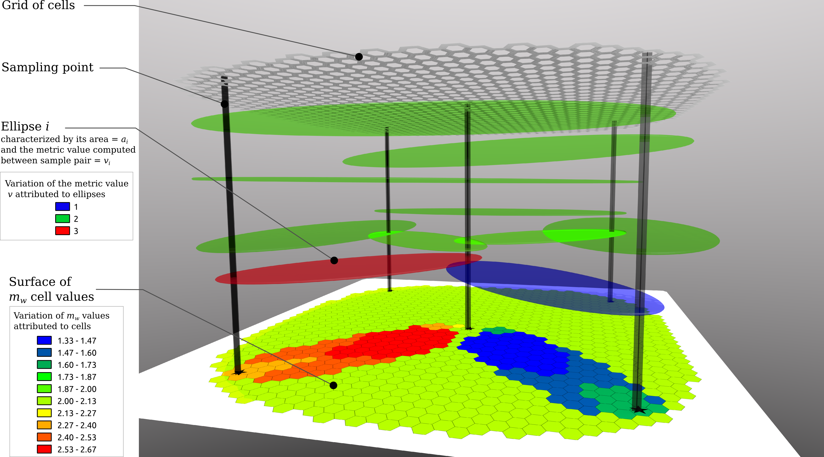
Figure 1: Schematic principle of the MAPI method from Piry et al. 2016.
Input data
The analysis requires two tables (data.frame or data.table):
Information on samples: table with three mandatory columns and column names: 'ind' (sample name), 'x' and 'y' (projected coordinates). An optional column 'errRad' (radius of error circle on sample coordinates) can be provided.
MAPI requires cartesian coordinates (ie. projected, such as UTM or Lambert) NOT (yet?) angular coordinates (eg. latitude/longitude).
The package sf provides the st_transform function for coordinates transformation and projection.
GIS software such as QGis can also help with datum transformation.
Example of 'samples' data:
| ind | x | y | errRad | |
| 1 | 2_42 | 12000 | 5000 | 10 |
| 2 | 2_47 | 17000 | 5000 | 10 |
| 3 | 1_82 | 2000 | 9000 | 10 |
| 4 | 2_100 | 20000 | 10000 | 10 |
| 5 | 2_87 | 17000 | 9000 | 10 |
| 6 | 1_11 | 1000 | 2000 | 10 |
| ... | ... | ... | ... | ... |
Values of the pairwise metric computed between samples provided, either, as a complete matrix with the same number of columns and rows (column and row names must match the sample names provided in the 'samples' data) or as a table with three mandatory columns and column names: 'ind1', 'ind2' (sample names) and 'value' (pairwise metric values).
Example of 'metric' data:
| ind1 | ind2 | value | |
| 1 | 1_1 | 1_2 | 0.055556 |
| 2 | 1_1 | 1_3 | 0.020833 |
| 3 | 1_1 | 1_4 | 0.125000 |
| 4 | 1_1 | 1_5 | 0.125000 |
| 5 | 1_1 | 1_6 | 0.020833 |
| 6 | 1_1 | 1_7 | 0.090278 |
| ... | ... | ... | ... |
Try it
Using the test dataset ('samples' and 'metric') included in the package, let's run an (almost) automatic MAPI analysis
Test data result from population genetic simulations in which two panmictic populations are separated by a barrier to dispersal. As we use dummy coordinates, there is no appropriate crs, so we just use 'crs=3857' (a pseudo-mercator projection). Of course, in this case, sample position on earth is meaningless. For a real dataset, 'crs' must be the EPSG code of the projection of your cartesian coordinates.
 # Load the package
 library(mapi)

 # Load 'samples' data
 data("samples")

 # Load 'metric' data. For our simulated data set the parwise metric
 # computed between samples is the individual genetic distance â of Rousset (2000).
 data("metric")

 # Run MAPI the lazy way (automatic) with 1000 permutations
 # for detection of significant (dis)continuous areas.
 # As crs must be set, we go with crs=3857 even if we use dummy coordinates.
 # Of course, this have no geographical meaning.
 # As we have a regular sampling, we use beta=0.5
 my.results <- MAPI_RunAuto(samples, metric, crs=3857, beta=0.5, nbPermuts=1000)

 # Get significant areas with a FDR control at alpha=0.05 (5%, by default)
 my.tails <- MAPI_Tails(my.results, alpha=0.05)

 # Look at the result Figure 2.
 MAPI_Plot2(my.results, tails=my.tails)
Spatial variation of the genetic distance is represented with a color scale from dark brown (lowest values) to dark blue (higher value). The central blue area identified as a significant area of discontinuity corresponds to the position of the simulated barrier. Note that due to the permutation procedure, delineation of the significant areas may vary slightly among runs.
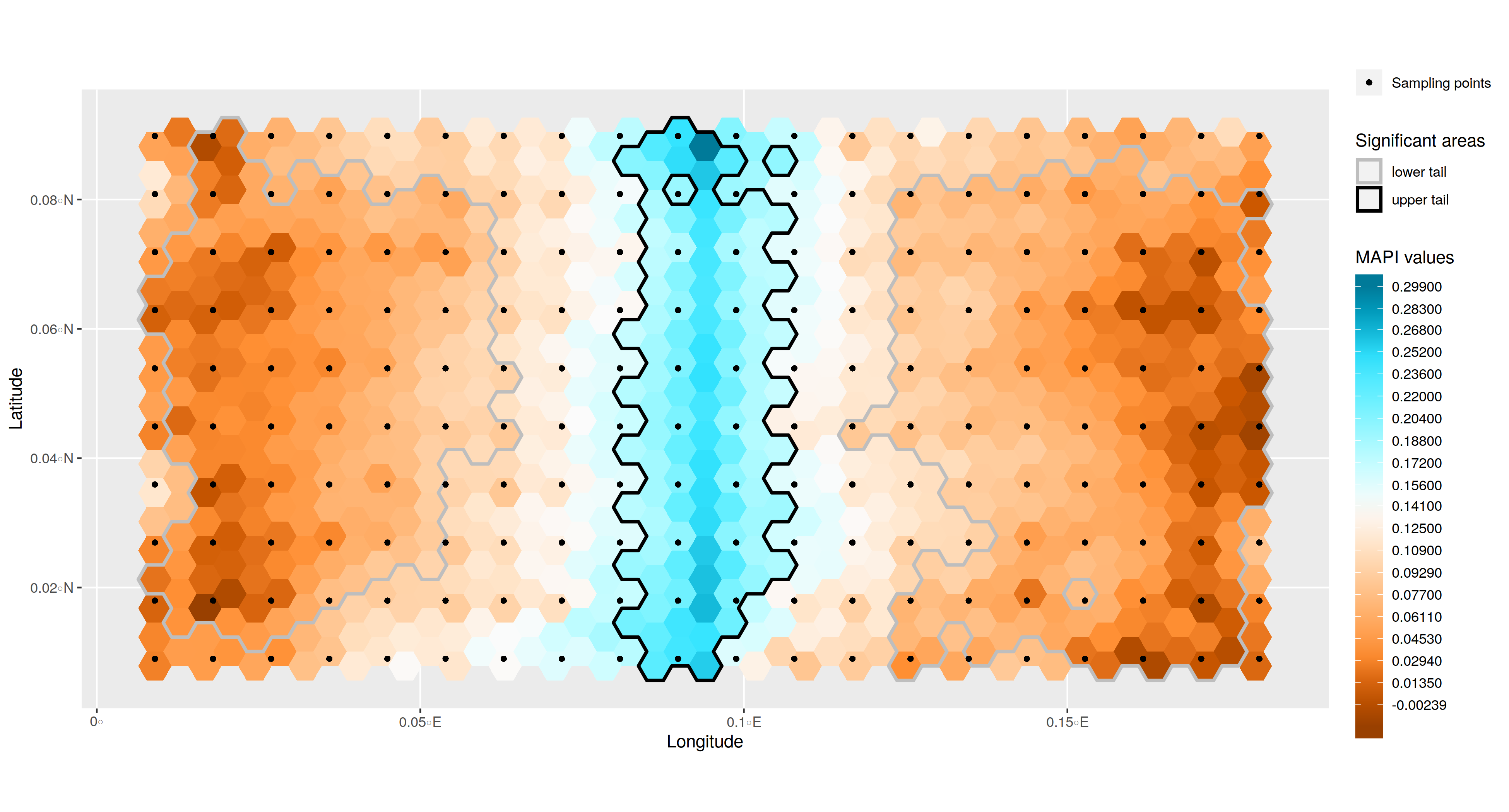
Figure 2: MAPI graphical Output produced using the MAPI_Plot2 function.
To go deeper
MAPI_RunAuto is a wrapper which calls three other functions: MAPI_CheckData, MAPI_GridAuto and MAPI_RunOnGrid.
MAPI_GridAuto is itself another wrapper around MAPI_EstimateHalfwidth and MAPI_GridHexagonal.
Typically, a "manual" MAPI analysis will involve the following ordered steps:
Within this general framework, you may, for example:
set your own value for 'halfwidth' (ignore step 2)
use your own grid, or reuse one from another run (ignore steps 2 & 3)
tweak some MAPI parameters (such as dMin or dMax for filtering on geographic distances between samples)
discard poorly supported cells prior detecting significant areas of (dis)continuity (parameter
minQ) and/or change significance level (parameteralphainMAPI_Tails)build your MAPI maps with a GIS software (ignore step 6). See 'Export results' section below
Export results
Output tables (weighted mean of the pairwise metric within cell and polygons delineating significant areas of (dis)continuity) are spatial objects built using the package sf.
Refer to sf documentation to export MAPI results in various format.
Below is an example of how MAPI results can be exported as ESRI Shapefiles:
library(sf)
# Export results for our test dataset
st_write(my.results, dsn=".", layer="myFirstMapiResult",
   driver="ESRI Shapefile", update=TRUE, delete_layer=TRUE)
st_write(my.tails, dsn=".", layer="myFirstMapiResultTails",
   driver="ESRI Shapefile", update=TRUE, delete_layer=TRUE)
You may now open these files ‘myFirstMapiResult.shp’ and ‘myFirstMapiResultTails.shp’ in a GIS software such as QGis and customize the layout.
Overlaying MAPI results with landscape layouts can help in analyzing the relationship between environmental features and spatial genetic patterns (eg. Piry et al., 2016; Piry et al., 2018).
References
Description of the MAPI method
Piry S., Chapuis M.-P., Gauffre B., Papaïx J., Cruaud A. and Berthier K. (2016).
Mapping Averaged Pairwise Information (MAPI): a new exploratory tool to uncover spatial structure.
Methods in Ecology and Evolution 7:(12), 1463–1475.
doi:10.1111/2041-210X.12616
Applications of MAPI in Landscape Genetics
Larson S., Gagne RB et al. 2021 Translocations maintain genetic diversity and increase connectivity in sea otters, Enhydra lutris Marine Mammal Science doi:10.1111/mms.12841
Stragier C., Piry S., et al. 2020. Interplay between historical and current features of the cityscape in shaping the genetic structure of the house mouse (Mus musculus domesticus) in Dakar (Senegal, West Africa) bioRxiv ; Version 4 of this preprint has been peer-reviewed and is recommended by Peer Community In Ecology (DOI:10.24072/pci.ecology.100044) doi:10.1101/557066
Piry S., Berthier K., Streiff R., Cros-Arteil S., Tatin L., Foucart A., Bröder L., Hochkirch A., and Chapuis M.-P. (2018). Fine-scale interactions between habitat quality and genetic variation suggest an impact of grazing on the critically endangered Crau Plain grasshopper (Pamphagidae: Prionotropis rhodanica). Journal of Orthoptera Research 27, 61–73. doi:10.3897/jor.27.15036
Dellicour S, Prunier JG, Piry S, et al. (2019) Landscape genetic analyses of Cervus elaphus and Sus scrofa: comparative study and analytical developments. Heredity. doi:10.1038/s41437-019-0183-5
Function MAPI_CheckData
Description
Check the validity of the 'samples' and 'metric' data loaded.
Missing data are removed from 'metric', samples with missing coordinates are removed and samples that are not present in both dataset ('samples' and 'metric') are discarded.
Usage
MAPI_CheckData(
  samples,
  metric,
  isMatrix = all(("matrix" %in% class(metric)), (nrow(metric) == ncol(metric)))
)
Arguments
samples |
a data.frame with names and geographical coordinates of samples. Column names must be: 'ind', 'x', 'y'. Optional column 'errRad' with an error radius for sample locations (eg. GPS uncertainty). Coordinates must be projected (not latitude/longitude). |
metric |
a data.frame or a square matrix with the pairwise metric computed for all pairs of samples. If data.frame, column names must be: 'ind1', 'ind2', 'value'. If matrix, sample names must be the row- and column names. |
isMatrix |
Boolean. Depends on the 'metric' data: |
Value
a list of two data.table objects corresponding to 'samples' and 'metric' after cleaning.
Examples
## Not run:
data("samples")
data("metric")
# remove first sample in order to force warning
samples <- samples[-c(1) , ]
clean.list <- MAPI_CheckData(samples, metric)
checked.samples <- clean.list[['samples']]
checked.metric <- clean.list[['metric']]

## End(Not run)
Function MAPI_EstimateHalfwidth
Description
This function computes the side length (= halfwidth) of the hexagonal cells. Halfwidth value can be further used to build a MAPI grid.
Usage
MAPI_EstimateHalfwidth(samples, crs, beta = 0.25)
Arguments
samples |
a data.frame with names and geographical coordinates of samples. Column names must be: 'ind', 'x', 'y'. Optional column 'errRad' with an error radius for sample locations (eg. GPS uncertainty). Coordinates must be projected (not latitude/longitude). |
crs |
coordinate reference system: integer with the EPSG code, or character with proj4string. The coordinates system must be a projection, not latitude/longitude. |
beta |
A value depending on spatial regularity of sampling: 0.5 for regular sampling, 0.25 for random sampling (Hengl, 2006). |
Details
h_w = \frac{\beta \sqrt{A/N}}{\sqrt{2.5980}}, where A is the study area (convex hull of sampling points) and N the number of samples.
Parameter beta allows to respect the Nyquist-Shannon sampling theorem depending on sampling regularity.
Value
halfwidth cell value (side length of hexagonal cells).
References
Hengl, T. (2006) Finding the right pixel size. Computers & Geosciences, 32, 1283–1298.
Examples
data(samples)
# Computes hexagonal cell halfwidth for the 'samples' dataset using beta=0.5
hw <- MAPI_EstimateHalfwidth(samples, crs=3857, beta=0.5)
Function MAPI_GridAuto
Description
Wrapper that computes cell halfwidth for a given beta value, and then
builds a grid of hexagonal cells (call to MAPI_GridHexagonal).
If coordinates are in angular units (eg. longitude/latitude) MAPI will try to build a worldwide
"discrete global grid system" using package 'dggridR'.
As the 'dggridR' package is no more available on CRAN, this feature have been removed
and an error is thrown in this case.
See https://github.com/r-barnes/dggridR for more informations.
As an alternative, grids (levels 1 to 11) are downloadable from MAPI website.
Usage
MAPI_GridAuto(samples, crs, beta = 0.25, buf = 0)
Arguments
samples |
a data.frame with names and geographical coordinates of samples. Column names must be: 'ind', 'x', 'y'. If coordinates are angular (ie. latitude/longitude), note that x stands for the longitude and y for the latitude. Optional column 'errRad' with an error radius for sample locations (eg. GPS uncertainty). |
crs |
coordinate reference system: integer with the EPSG code, or character with proj4string. When using dummy coordinates (eg. simulation output) you may use EPSG:3857 (pseudo-Mercator) for example. This allows computation but, of course, has no geographical meaning. |
beta |
A value depending on sampling regularity: 0.5 for regular sampling, 0.25 for random sampling (Hengl, 2006). |
buf |
optional. This parameter allows to expand or shrink the grid by a number of units in the same reference system as the sample geographical coordinates (0 by default). |
Details
The halfwidth cell value used to build the grid is computed as
h_w = \frac{\beta \sqrt{A/N}}{\sqrt{2.5980}},
where A is the study area (convex hull of sampling points) and N the number of samples.
Parameter beta allows to respect the Nyquist-Shannon sampling theorem depending on sampling regularity
(call to MAPI_EstimateHalfwidth).
If coordinates are provided as longitude/latitude (eg. crs=4326) MAPI will try to build a worldwide grid.
See MAPI_EstimateHalfwidth and MAPI_GridHexagonal for more information.
Value
a spatial object of class 'sf' including the x and y coordinates of cell centers, cell geometry (polygons) and cell id (gid).
Examples
data("samples")
grid <- MAPI_GridAuto(samples, crs=3857, beta=0.5)
Function MAPI_GridHexagonal
Description
Build a grid of hexagonal cells according to samples coordinates and a given halfwidth
cell value provided by users (can be computed using MAPI_EstimateHalfwidth).
If coordinates are in angular units (eg. longitude/latitude) MAPI will try to build a worldwide
"discrete global grid system" using package 'dggridR'.
As the 'dggridR' package is no more available on CRAN, this feature have been removed
and an error is thrown in this case.
See https://github.com/r-barnes/dggridR for more informations.
As an alternative, grids (levels 1 to 11) are downloadable from MAPI website.
Usage
MAPI_GridHexagonal(samples, crs, hw, buf = 0)
Arguments
samples |
a data.frame with names and geographical coordinates of samples. Column names must be: 'ind', 'x', 'y'. Optional column 'errRad' with an error radius for sample locations (eg. GPS uncertainty). |
crs |
coordinate reference system: integer with the EPSG code, or character with proj4string. When using dummy coordinates (eg. simulation output) you may use EPSG:3857 for example. This allows computation but, of course, has no geographical meaning. |
hw |
Halfwidth : side length of hexagonal cells. |
buf |
optional. This parameter allows to expand or shrink the grid by a number of units in the same reference system as the sample geographical coordinates (0 by default, ignored for worldwide grids). |
Value
a spatial object of class 'sf' including the x and y coordinates of cell centers, cell geometry (polygons) and cell id (gid).
Examples
data("samples")
# Builds a grid of hexagonal cells according to samples coordinates (columns x and y)
# using the EPSG:3857 projection and an halfwidth cell value of hw=250m.
grid <- MAPI_GridHexagonal(samples, crs=3857, hw=250)
Function MAPI_Plot
Description
Plot a MAPI analysis result
Usage
MAPI_Plot(
  resu,
  tails = NULL,
  samples = NULL,
  pal = c("#994000", "#CC5800", "#FF8F33", "#FFAD66", "#FFCA99", "#FFE6CC", "#FBFBFB",
    "#CCFDFF", "#99F8FF", "#66F0FF", "#33E4FF", "#00AACC", "#007A99"),
  shades = 20,
  main = NA,
  upper = TRUE,
  lower = TRUE,
  upper.border = "black",
  lower.border = "gray"
)
Arguments
resu |
A spatial object of class 'sf' resulting from a MAPI analysis done using
|
tails |
An optional spatial object of class 'sf' resulting from the post-process with
|
samples |
A data.frame with names and geographical coordinates of samples. Column names must be: 'ind', 'x', 'y'. Optional column 'errRad' with an error radius for sample locations (eg. GPS uncertainty). Coordinates must be projected (not latitude/longitude). |
pal |
A color ramp, eg. from RColorBrewer (default: orange > light gray > blue) |
shades |
Number of breaks for the color ramp (default 20) |
main |
Plot title (none by default) |
upper |
If TRUE and tails is not NULL, upper-tail significant areas are plotted. TRUE by default. |
lower |
If TRUE and tails is not NULL, lower-tail significant areas are plotted. TRUE by default. |
upper.border |
Border color of the upper-tail significant area. "black" by default. |
lower.border |
Border color of the lower-tail significant area. "gray" by default. |
Value
Returns the "trellis" object.
Examples
## Not run:
data("metric")
data("samples")
resu <- MAPI_RunAuto(samples, metric, crs=3857, nbPermuts = 1000)
tails <- MAPI_Tails(resu)
pl <- MAPI_Plot(resu, tails=tails, samples=samples)
# Open png driver
png("mapiPlotOutput.png", width=1000, type="cairo-png")
print(pl) # Do plot in file
dev.off() # Close driver

## End(Not run)
Function MAPI_Plot2
Description
Plot a MAPI analysis result with ggplot
Usage
MAPI_Plot2(
  resu,
  tails = NULL,
  samples = NULL,
  pal = c("#994000", "#CC5800", "#FF8F33", "#FFAD66", "#FFCA99", "#FFE6CC", "#FBFBFB",
    "#CCFDFF", "#99F8FF", "#66F0FF", "#33E4FF", "#00AACC", "#007A99"),
  shades = 20,
  main = "",
  upper = TRUE,
  lower = TRUE,
  upper.border = "black",
  lower.border = "gray"
)
Arguments
resu |
A spatial object of class 'sf' resulting from a MAPI analysis done using
|
tails |
An optional spatial object of class 'sf' resulting from the post-process with
|
samples |
A data.frame with names and geographical coordinates of samples. Column names must be: 'ind', 'x', 'y'. Optional column 'errRad' with an error radius for sample locations (eg. GPS uncertainty). Coordinates must be projected (not latitude/longitude). |
pal |
A color ramp, eg. from RColorBrewer (default: orange > light gray > blue) |
shades |
Number of breaks for the color ramp (default 20) |
main |
Plot title (none by default) |
upper |
If TRUE and tails is not NULL, upper-tail significant areas are plotted. TRUE by default. |
lower |
If TRUE and tails is not NULL, lower-tail significant areas are plotted. TRUE by default. |
upper.border |
Border color of the upper-tail significant area. "black" by default. |
lower.border |
Border color of the lower-tail significant area. "gray" by default. |
Value
Returns the ggplot object.
Examples
## Not run:
library(ggplot2)
data("metric")
data("samples")
resu <- MAPI_RunAuto(samples, metric, crs=3857, nbPermuts = 1000)
tails <- MAPI_Tails(resu)
pl <- MAPI_Plot2(resu, tails=tails, samples=samples)
# Save to image
ggsave("mapiPlotOutput.png", plot=pl)

## End(Not run)
Function MAPI_RunAuto
Description
This function is a wrapper allowing to run a complete MAPI analysis.
Usage
MAPI_RunAuto(
  samples,
  metric,
  crs,
  isMatrix = all(class(metric) == "matrix", nrow(metric) == ncol(metric)),
  beta = 0.25,
  ecc = 0.975,
  buf = 0,
  errRad = 10,
  nbPermuts = 0,
  dMin = 0,
  dMax = Inf,
  nbCores = ifelse(requireNamespace("parallel", quietly = TRUE), parallel::detectCores()
    - 1, 1),
  N = 8
)
Arguments
samples |
a data.frame with names and geographical coordinates of samples. Column names must be: 'ind', 'x', 'y'. Optional column 'errRad' with an error radius for sample locations (eg. GPS uncertainty). Coordinates must be projected (not latitude/longitude). |
metric |
a data.frame or a square matrix with the pairwise metric computed for all pairs of samples. If data.frame, column names must be: 'ind1', 'ind2', 'value'. If matrix, sample names must be the row- and column names. |
crs |
coordinate reference system: integer with the EPSG code, or character with proj4string. When using dummy coordinates (eg. simulation output) you may use EPSG:3857 for example. This allows computation but, of course, has no geographical meaning. |
isMatrix |
Boolean. Depends on the 'metric' data: |
beta |
A value depending on spatial regularity of sampling: 0.5 for regular sampling, 0.25 for random sampling (Hengl, 2006). |
ecc |
ellipse eccentricity value (0.975 by default). |
buf |
optional. This parameter allows to expand or shrink the grid by a number of units in the same reference system as the sample geographical coordinates (0 by default). |
errRad |
global error radius for sample locations (same radius for all samples, 10 by default).
Units are in the same reference system as the sample geographical coordinates.
To use different error radius values for sample locations, add a column 'errRad' in the 'sample' data (see |
nbPermuts |
number of permutations of sample locations (0 by default). |
dMin |
minimum distance between individuals. 0 by default. |
dMax |
maximal distance between individuals. +Inf by default. |
nbCores |
number of CPU cores you want to use during parallel computation. The default value is estimated as the number of available cores minus 1, suitable for a personal computer. On a cluster you might have to set it to a reasonable value (eg. 8) in order to keep resources for other tasks. |
N |
number of points used per quarter of ellipse, 8 by default. Don't change it unless you really know what you are doing. |
Details
Following functions are called by MAPI_RunAuto in following order:
-
MAPI_CheckDatacleans the dataset; -
MAPI_GridAutogenerates a grid of hexagons by callingMAPI_EstimateHalfwidththenMAPI_GridHexagonal; -
MAPI_RunOnGridperforms the MAPI analysis.
NOTE: The call to MAPI_Tails is not included.
It should be done afterwards on the object returned by MAPI_RunAuto.
Value
a spatial object of class 'sf' providing for each cell:
gid: Cell ID
x and y coordinates of cell center
nb_ell: number of ellipses used to compute the weighted mean
avg_value: weighted mean of the pairwise metric
sum_wgts: sum of weights of ellipses used to compute the weighted mean
w_stdev: weighted standard deviation of the pairwise metric
swQ: percentile of the sum of weights
geometry
When permutations are performed:
proba: proportion of the permuted weighted means below the observed weighted mean
ltP: lower-tail p-value adjusted using the FDR procedure of Benjamini and Yekutieli
utP: upper-tail p-value adjusted using the FDR procedure of Benjamini and Yekutieli
References
Benjamini, Y. & Yekutieli, D. (2001) The control of the false discovery rate in multiple testing under dependency. Annals of Statistics, 29, 1165–1188.
Examples
## Not run:
data("metric")
data("samples")
# Run a MAPI analysis without permutation
my.results <- MAPI_RunAuto(samples, metric, crs=3857, beta=0.5, nbPermuts=0)

# eg. Export results to shapefile "myFirstMapiResult" in current directory
# to further visualize and customize the MAPI plot in SIG software.
library(sf)
st_write(my.results, dsn=".", layer="myFirstMapiResult", driver="ESRI Shapefile")

## End(Not run)
Function MAPI_RunOnGrid
Description
Launch a MAPI analysis for a given grid computed with MAPI_GridAuto
or MAPI_GridHexagonal or provided by users.
Usage
MAPI_RunOnGrid(
  samples,
  metric,
  grid,
  isMatrix = FALSE,
  ecc = 0.975,
  errRad = 10,
  nbPermuts = 0,
  dMin = 0,
  dMax = Inf,
  use_s2 = FALSE,
  nbCores = parallel::detectCores() - 1,
  N = 8,
  ignore.weights = FALSE
)
Arguments
samples |
a data.frame with names and geographical coordinates of samples. Column names must be: 'ind', 'x', 'y'. Optional column 'errRad' with an error radius for sample locations (eg. GPS uncertainty). Coordinates should be projected (not latitude/longitude) for a local dataset, angular coordinates (ie. latitude/longitude) are accepted for worldwide datasets. In this case, the longitude will be in the "x" column and the latitude in the "y" column. |
metric |
a data.frame or a square matrix with the pairwise metric computed for all pairs of samples. If data.frame, column names must be: 'ind1', 'ind2', 'value'. If matrix, sample names must be the row- and column names. |
grid |
a spatial object of class 'sf' with the geometry of each cell.
When using your own grid, please check that the object structure is the same as returned by
|
isMatrix |
Boolean. Depends on the 'metric' data: |
ecc |
ellipse eccentricity value (0.975 by default). |
errRad |
global error radius for sample locations (same radius for all samples, 10 by default).
Units are in the same reference system as the sample geographical coordinates.
To use different error radius values for sample locations, add a column 'errRad' in the 'sample' data (see |
nbPermuts |
number of permutations of sample locations (0 by default). |
dMin |
minimum distance between individuals. 0 by default. |
dMax |
maximal distance between individuals. +Inf by default. |
use_s2 |
transform grid and coordinates in latitude,longitude in order to use s2 library functions (default FALSE). When set to TRUE mapi is able to process worldwide grids and ellipses and generate results on the sphere. |
nbCores |
number of CPU cores you want to use during parallel computation. The default value is estimated as the number of available cores minus 1, suitable for a personal computer. On a cluster you might have to set it to a reasonable value (eg. 8) in order to keep resources for other tasks. |
N |
number of points used per quarter of ellipse, 8 by default. Don't change it unless you really know what you are doing. |
ignore.weights |
allow to compute a simple mean instead of the default weighted mean. This implies that all ellipses bear the same weight. |
Details
To test whether the pairwise metric values associated with the ellipses are independent of the sample locations, those are permuted 'nbPermuts' times. At each permutation, new cell values are computed and stored to build a cumulative null distribution for each cell of the grid. Each cell value from the observed data set is then ranked against its null distribution. For each cell, the proportion of permuted values that are smaller or greater than the observed value provides a lower-tailed (ltP) and upper-tailed (utP) test p-value.
A false discovery rate (FDR) procedure (Benjamini and Yekutieli, 2001) is applied to account for multiple
testing (number of cells) under positive dependency conditions (spatial autocorrelation). An adjusted
p-value is computed for each cell using the function p.adjust from the 'stats' package with the method 'BY'.
Value
a spatial object of class 'sf' providing for each cell:
gid: Cell ID
x and y coordinates of cell center
nb_ell: number of ellipses used to compute the weighted mean
avg_value: weighted mean of the pairwise metric
sum_wgts: sum of weights of ellipses used to compute the weighted mean
w_stdev: weighted standard deviation of the pairwise metric
swQ: percentile of the sum of weights
geometry
When permutations are performed:
proba: proportion of the permuted weighted means below the observed weighted mean
ltP: lower-tail p-value adjusted using the FDR procedure of Benjamini and Yekutieli
utP: upper-tail p-value adjusted using the FDR procedure of Benjamini and Yekutieli
References
Benjamini, Y. and Yekutieli, D. (2001). The control of the false discovery rate in multiple testing under dependency. Annals of Statistics 29, 1165–1188.
Examples
## Not run:
data(metric)
data(samples)
my.grid <- MAPI_GridHexagonal(samples, crs=3857, 500) # 500m halfwidth

# Note: 10 permutations is only for test purpose, increase to >=1000 in real life!
my.results <- MAPI_RunOnGrid(samples, metric, grid=my.grid, nbPermuts=10, nbCores=1)

# eg. Export results to shapefile "myFirstMapiResult" in current directory
sf::st_write(my.results, dsn=".", layer="myFirstMapiResult", driver="ESRI Shapefile")

## End(Not run)
Function MAPI_Tails
Description
Determine significant continuous and discontinuous areas from the result of a MAPI analysis when run with permutations.
Usage
MAPI_Tails(resu, minQ = 0, alpha = 0.05)
Arguments
resu |
A spatial object of class 'sf' resulting from a MAPI analysis done using either
|
minQ |
Threshold under which cells with the smallest sum-of-weights percentile (range 1 .. 100) are discarded (default value = 0). This parameter allows to discard cells for which the average value of the pairwise metric is computed using either a small number and/or only long-distance ellipses. |
alpha |
Significance level (default=0.05) |
Details
When permutations are performed, in MAPI_RunOnGrid for each cell, the proportion of permuted values that are smaller or greater
than the observed value provides a lower-tailed (ltP) and upper-tailed (utP) test p-value.
A false discovery rate (FDR) procedure (Benjamini and Yekutieli, 2001) is applied to account for multiple
testing (number of cells) under positive dependency conditions (spatial autocorrelation). An adjusted
p-value is computed for each cell using the function p.adjust from the 'stats' package with the method 'BY'.
The significance level at which FDR is controlled is set through the parameter alpha. For example, when alpha is
set to 0.05, this means that 5\
Significant cells belonging to the lower (or upper) tail that are spatially connected are aggregated together to form the significant areas with the lowest (or greater) average values of the pairwise metric analyzed.
Value
a spatial object of class 'sf' with the area and geometry of the polygons delineating the significant areas. A column provides the tail for each polygon (upper or lower).
References
Benjamini, Y. and Yekutieli, D. (2001). The control of the false discovery rate in multiple testing under dependency. Annals of Statistics 29, 1165–1188.
Examples
## Not run:
data("metric")
data("samples")
# Run MAPI computation
resu <- MAPI_RunAuto(samples, metric, crs=3857, nbPermuts=1000)
# Discards the 10% cells with the smallest sum-of-weights
#    and aggregates adjacent cells belonging to the same tail
#    at a 5% significance level
tails <- MAPI_Tails(resu, minQ=10, alpha=0.05)

## End(Not run)
Function MAPI_Varicell
Description
Alter grid by changing polygons size according to samples density.
Usage
MAPI_Varicell(grid, samples, buf = 0, var.coef = 50)
Arguments
grid |
a spatial object of class 'sf' with the geometry of each cell.
When using your own grid, please check that the object structure is the same as returned by
|
samples |
a data.frame with names and geographical coordinates of samples. Column names must be: 'ind', 'x', 'y'. Optional column 'errRad' with an error radius for sample locations (eg. GPS uncertainty). Coordinates must be projected (not latitude/longitude) and in the same projection as the grid. |
buf |
This parameter allows to clip the grid around samples by a number of units in the same reference system as the grid geographical coordinates (0 by default). A value 3-5 times smaller than the size used to build the grid may be OK. |
var.coef |
optional, default value=50. The expected ratio of size between largest and smallest cells in final grid. |
Value
a spatial object of class 'sf' including cell area, the x and y coordinates of cell centroids, cell geometry (polygons) and cell id (gid) plus the computed densities and weights.
Examples
## Not run:
# Dummy example!
require(data.table, sf, mapi, spatstat.geom, spatstat.core)
data("samples")
keep <- c(2,3,6,9,10,11,16,18,19,20,21,23,26,27,29,31,33,34,38,41,46,50,54,58,61,63,65,71,72,73,
76,78,79,81,85,92,93,94,97,98,99,101,103,113,115,119,120,121,124,127,130,134,142,143,151,152,159,
160,176,185,189,191,195,196,197,198,199)
samples2 <- samples[keep, ] # keep only one third in order to create discontinuities
set.seed(1234)
# Builds a grid of hexagonal cells according to samples coordinates (columns x and y)
# using the EPSG:3857 projection and an halfwidth cell value of hw=250m.
grid <- MAPI_GridHexagonal(samples2, crs=3857, hw=250, buf=1500)
grid.var <- MAPI_Varicell(grid, samples2, buf=250, var.coef=20)
ggplot() +
    geom_sf(data=grid.var, aes(fill=dens), size=0.1) +
    geom_sf(data=st_as_sf(samples2, coords=c("x","y"), crs=3857), aes())

## End(Not run)
'metric' test dataset
Description
The individuals were simulated as described in the samples section.
The value is a genetic distance (â estimator in Rousset, 2000) computed between the
200 simulated samples using SPAGeDi v1.4 (Hardy & Vekemans, 2002).
Usage
data("metric")
Value
A data.table object with 19900 rows (one per sample pair, non symmetrical) and 3 columns ("ind1", "ind2", "value") containing respectively the first sample name, the second sample name and the value of their relation.
References
Rousset, F. (2000). Genetic differentiation between individuals. Journal of Evolutionary Biology, 13:58–62.
Hardy OJ, Vekemans X (2002) SPAGeDi: a versatile computer program to analyse spatial genetic structure at the individual or population levels. Molecular Ecology Notes 2: 618-620.
Examples
data("metric")
'samples' test dataset
Description
Test dataset provided with the MAPI package. We used generation-by-generation coalescent algorithms (Hudson et al., 1990) to simulate 10 microsatellite genotypes at migration-mutation-drift equilibrium for 200 diploid individuals, distributed on the nodes of a 20x10 lattice.
Mutations for each locus followed a symmetric generalized stepwise model with a variance equal to 0.36 (Estoup et al., 2001) and a maximum range of allelic states of 40. The mutation rate was fixed so that heterozygosity ranged from 0.6 to 0.8 as frequently observed at microsatellite markers (Chapuis et al., 2012).
Two panmictic populations are separated by a barrier. We used
Simcoal2 (Laval and Excoffier, 2004) to generate two panmictic populations of equal effective size
N_e = 100 and exchanging N_{e}m = 0.1 migrants at each generation. The barrier to gene
flow bisected the lattice from north to south in its center.
The differentiation values computed between these samples is described in the metric section.
Usage
data("samples")
Value
A data.table object with 200 simulated individuals (one per row) and 4 columns ("ind", "x", "y", "errRad") including the sample names, coordinates x and y and an error circle radius on coordinates.
References
Chapuis, M.-P., Streiff, R., and Sword, G. (2012). Long microsatellites and unusually high levels of genetic diversity in the orthoptera. Insect Molecular Biology, 21(2):181–186.
Estoup, A., Wilson, I. J., Sullivan, C., Cornuet, J.-M., and Moritz, C. (2001). Inferring population history from microsatellite and enzyme data in serially introduced cane toads, Bufo marinus. Genetics, 159(4):1671–1687.
Hudson, R. R. et al. (1990). Gene genealogies and the coalescent process. Oxford Surveys in Evolutionary Biology, 7(1):44.
Laval, G. and Excoffier, L. (2004). SIMCOAL 2.0: a program to simulate genomic diversity over large recombining regions in a subdivided population with a complex history. Bioinformatics, 20(15):2485–2487.
Examples
data("samples")