| Title: | Tidy Plots for Scientific Papers |
| Version: | 0.4.0 |
| Description: | The goal of 'tidyplots' is to streamline the creation of publication-ready plots for scientific papers. It allows to gradually add, remove and adjust plot components using a consistent and intuitive syntax. |
| License: | MIT + file LICENSE |
| Encoding: | UTF-8 |
| RoxygenNote: | 7.3.3 |
| Imports: | cli, dplyr, forcats, ggbeeswarm, ggplot2 (≥ 4.0.1), ggpubr, ggrastr, ggrepel, glue, gtable, Hmisc, htmltools, lifecycle, purrr, rlang, scales, stringr, tidyr, tidyselect |
| Depends: | R (≥ 4.1.0) |
| LazyData: | true |
| URL: | https://github.com/jbengler/tidyplots, https://jbengler.github.io/tidyplots/ |
| BugReports: | https://github.com/jbengler/tidyplots/issues |
| Suggests: | knitr, rmarkdown, testthat (≥ 3.0.0), vdiffr |
| VignetteBuilder: | knitr |
| Config/testthat/edition: | 3 |
| NeedsCompilation: | no |
| Packaged: | 2026-01-06 14:23:19 UTC; janbroderengler |
| Author: | Jan Broder Engler  [aut, cre, cph]
 |
| Maintainer: | Jan Broder Engler <broder.engler@gmail.com> |
| Repository: | CRAN |
| Date/Publication: | 2026-01-08 08:40:07 UTC |
tidyplots: Tidy Plots for Scientific Papers
Description
The goal of 'tidyplots' is to streamline the creation of publication-ready plots for scientific papers. It allows to gradually add, remove and adjust plot components using a consistent and intuitive syntax.
Author(s)
Maintainer: Jan Broder Engler broder.engler@gmail.com (ORCID) [copyright holder]
See Also
Useful links:
Report bugs at https://github.com/jbengler/tidyplots/issues
The pipe
Description
The pipe
Usage
lhs %>% rhs
Arguments
lhs |
A value. |
rhs |
A function call. |
Value
The result of the calling the function rhs with the parameter lhs.
Add ggplot2 code to a tidyplot
Description
Add ggplot2 code to a tidyplot
Usage
add()
Value
A tidyplot object.
Examples
study |>
  tidyplot(x = treatment, y = score, color = treatment) |>
  add(ggplot2::geom_point())
Add annotation
Description
Add annotation
Usage
add_annotation_text(plot, text, x, y, fontsize = 7, ...)

add_annotation_rectangle(
  plot,
  xmin,
  xmax,
  ymin,
  ymax,
  fill = plot$tidyplot$ink,
  color = NA,
  alpha = 0.1,
  ...
)

add_annotation_line(plot, x, xend, y, yend, color = plot$tidyplot$ink, ...)
Arguments
plot |
A |
text |
String for annotation text. |
x, xmin, xmax, xend, y, ymin, ymax, yend |
Coordinates for the annotation. |
fontsize |
Font size in points. Defaults to |
... |
Arguments passed on to |
fill |
A hex color for the fill color. For example, |
color |
A hex color for the stroke color. For example, |
alpha |
A |
Value
A tidyplot object.
Examples
study |>
  tidyplot(x = treatment, y = score, color = treatment) |>
  add_boxplot() |>
  add_annotation_text("Look here!", x = 2, y = 25)

eu_countries |>
  tidyplot(x = area, y = population) |>
  add_data_points() |>
  add_annotation_rectangle(xmin = 2.5e5, xmax = Inf, ymin = 42, ymax = Inf)

eu_countries |>
  tidyplot(x = area, y = population) |>
  add_data_points() |>
  add_annotation_rectangle(xmin = 2.5e5, xmax = 6e5, ymin = 42, ymax = 90,
                           color = "#E69F00", fill = NA)

eu_countries |>
  tidyplot(x = area, y = population) |>
  add_data_points() |>
  add_annotation_line(x = 0, xend = Inf, y = 0, yend = Inf)
Add area stack
Description
Add area stack
Usage
add_areastack_absolute(
  plot,
  linewidth = 0.25,
  alpha = 0.4,
  reverse = FALSE,
  replace_na = FALSE,
  ...
)

add_areastack_relative(
  plot,
  linewidth = 0.25,
  alpha = 0.4,
  reverse = FALSE,
  replace_na = FALSE,
  ...
)
Arguments
plot |
A |
linewidth |
Thickness of the line in points (pt). Typical values range between |
alpha |
A |
reverse |
Whether the order should be reversed or not. Defaults to |
replace_na |
Whether to replace |
... |
Arguments passed on to the |
Value
A tidyplot object.
Examples
# for a `count` provide `x` and `color`
# `count` of the data points in each `energy_type` category
energy |>
  tidyplot(x = year, color = energy_type) |>
  add_areastack_absolute()

energy |>
  tidyplot(x = year, color = energy_type) |>
  add_areastack_relative()

# for a `sum` provide `x`, `y` and `color`
# `sum` of `energy` in each `energy_type` category
energy |>
  tidyplot(x = year, y = energy, color = energy_type) |>
  add_areastack_absolute()

energy |>
  tidyplot(x = year, y = energy, color = energy_type) |>
  add_areastack_relative()

# Flip x and y-axis
energy |>
  tidyplot(x = energy, y = year, color = energy_type) |>
  add_areastack_absolute(orientation = "y")

energy |>
  tidyplot(x = energy, y = year, color = energy_type) |>
  add_areastack_relative(orientation = "y")
Add bar stack
Description
Add bar stack
Usage
add_barstack_absolute(plot, width = 0.8, reverse = FALSE, ...)

add_barstack_relative(plot, width = 0.8, reverse = FALSE, ...)
Arguments
plot |
A |
width |
Horizontal width of the plotted object (bar, error bar, boxplot,
violin plot, etc). Typical values range between |
reverse |
Whether the order should be reversed or not. Defaults to |
... |
Arguments passed on to the |
Value
A tidyplot object.
Examples
# for a `count` only provide `color`
# `count` of the data points in each `energy_type` category
energy |>
  tidyplot(color = energy_type) |>
  add_barstack_absolute()

energy |>
  tidyplot(color = energy_type) |>
  add_barstack_relative()

# for a `sum` provide `color` and `y`
# `sum` of `energy` in each `energy_type` category
energy |>
  tidyplot(y = energy, color = energy_type) |>
  add_barstack_absolute()

energy |>
  tidyplot(y = energy, color = energy_type) |>
  add_barstack_relative()

# Include variable on second axis
energy |>
  tidyplot(x = year, y = energy, color = energy_type) |>
  add_barstack_absolute()

energy |>
  tidyplot(x = year, y = energy, color = energy_type) |>
  add_barstack_relative()

# Flip x and y-axis
energy |>
  tidyplot(x = energy, y = year, color = energy_type) |>
  add_barstack_absolute(orientation = "y")

energy |>
  tidyplot(x = energy, y = year, color = energy_type) |>
  add_barstack_relative(orientation = "y")
Add boxplot
Description
Add boxplot
Usage
add_boxplot(
  plot,
  dodge_width = NULL,
  alpha = 0.3,
  saturation = 1,
  show_whiskers = TRUE,
  show_outliers = TRUE,
  box_width = 0.6,
  whiskers_width = 0.8,
  outlier.size = 0.5,
  coef = 1.5,
  outlier.shape = 19,
  outlier.alpha = 1,
  linewidth = 0.25,
  preserve = "total",
  ...
)
Arguments
plot |
A |
dodge_width |
For adjusting the distance between grouped objects. Defaults
to |
alpha |
A |
saturation |
A |
show_whiskers |
Whether to show boxplot whiskers. Defaults to |
show_outliers |
Whether to show outliers. Defaults to |
box_width |
Width of the boxplot. Defaults to |
whiskers_width |
Width of the whiskers. Defaults to |
outlier.size |
Size of the outliers. Defaults to |
coef |
Length of the whiskers as multiple of IQR. Defaults to 1.5. |
outlier.shape |
Shape of the outliers. Defaults to |
outlier.alpha |
Opacity of the outliers. Defaults to |
linewidth |
Thickness of the line in points (pt). Typical values range between |
preserve |
Should dodging preserve the |
... |
Arguments passed on to the |
Value
A tidyplot object.
Examples
study |>
  tidyplot(x = treatment, y = score, color = treatment) |>
  add_boxplot()

# Changing arguments:
study |>
  tidyplot(x = treatment, y = score, color = treatment) |>
  add_boxplot(show_whiskers = FALSE)

study |>
  tidyplot(x = treatment, y = score, color = treatment) |>
  add_boxplot(show_outliers = FALSE)

study |>
  tidyplot(x = treatment, y = score, color = treatment) |>
  add_boxplot(box_width = 0.2)

study |>
  tidyplot(x = treatment, y = score, color = treatment) |>
  add_boxplot(whiskers_width = 0.2)
Add count
Description
Add count
Usage
add_count_bar(
  plot,
  dodge_width = NULL,
  width = 0.6,
  saturation = 1,
  preserve = "total",
  ...
)

add_count_dash(
  plot,
  dodge_width = NULL,
  width = 0.6,
  linewidth = 0.25,
  preserve = "total",
  ...
)

add_count_dot(plot, dodge_width = NULL, size = 2, preserve = "total", ...)

add_count_value(
  plot,
  dodge_width = NULL,
  accuracy = 0.1,
  scale_cut = NULL,
  fontsize = 7,
  extra_padding = 0.15,
  vjust = NULL,
  hjust = NULL,
  preserve = "total",
  ...
)

add_count_line(
  plot,
  group,
  dodge_width = NULL,
  linewidth = 0.25,
  preserve = "total",
  ...
)

add_count_area(
  plot,
  group,
  dodge_width = NULL,
  linewidth = 0.25,
  preserve = "total",
  ...
)
Arguments
plot |
A |
dodge_width |
For adjusting the distance between grouped objects. Defaults
to |
width |
Horizontal width of the plotted object (bar, error bar, boxplot,
violin plot, etc). Typical values range between |
saturation |
A |
preserve |
Should dodging preserve the |
... |
Arguments passed on to the |
linewidth |
Thickness of the line in points (pt). Typical values range between |
size |
A |
accuracy |
A number to round to. Use (e.g.) Applied to rescaled data. |
scale_cut |
Scale cut function to be applied. See |
fontsize |
Font size in points. Defaults to |
extra_padding |
Extra padding to create space for the value label. |
vjust |
Vertical position adjustment of the value label. |
hjust |
Horizontal position adjustment of the value label. |
group |
Variable in the dataset to be used for grouping. |
Value
A tidyplot object.
Examples
dinosaurs |>
  tidyplot(x = time_lived, color = time_lived) |>
  adjust_x_axis(rotate_labels = TRUE) |>
  add_count_bar()

dinosaurs |>
  tidyplot(x = time_lived, color = time_lived) |>
  adjust_x_axis(rotate_labels = TRUE) |>
  add_count_dash()

dinosaurs |>
  tidyplot(x = time_lived, color = time_lived) |>
  adjust_x_axis(rotate_labels = TRUE) |>
  add_count_dot()

dinosaurs |>
  tidyplot(x = time_lived, color = time_lived) |>
  adjust_x_axis(rotate_labels = TRUE) |>
  add_count_value()

dinosaurs |>
  tidyplot(x = time_lived) |>
  adjust_x_axis(rotate_labels = TRUE) |>
  add_count_line()

dinosaurs |>
  tidyplot(x = time_lived) |>
  adjust_x_axis(rotate_labels = TRUE) |>
  add_count_area()

# Combination
dinosaurs |>
  tidyplot(x = time_lived) |>
  adjust_x_axis(rotate_labels = TRUE) |>
  add_count_bar(alpha = 0.4) |>
  add_count_dash() |>
  add_count_dot() |>
  add_count_value() |>
  add_count_line()

# Changing arguments: alpha
# Makes objects transparent
dinosaurs |>
  tidyplot(x = time_lived, color = time_lived) |>
  theme_minimal_y() |>
  adjust_x_axis(rotate_labels = TRUE) |>
  add_count_bar(alpha = 0.4)

# Changing arguments: saturation
# Reduces fill color saturation without making the object transparent
dinosaurs |>
  tidyplot(x = time_lived, color = time_lived) |>
  theme_minimal_y() |>
  adjust_x_axis(rotate_labels = TRUE) |>
  add_count_bar(saturation = 0.3)

# Changing arguments: accuracy
dinosaurs |>
  tidyplot(x = time_lived, color = time_lived) |>
  adjust_x_axis(rotate_labels = TRUE) |>
  add_count_value(accuracy = 1)

# Changing arguments: fontsize
dinosaurs |>
  tidyplot(x = time_lived, color = time_lived) |>
  adjust_x_axis(rotate_labels = TRUE) |>
  add_count_value(fontsize = 10)

# Changing arguments: color
dinosaurs |>
  tidyplot(x = time_lived, color = time_lived) |>
  adjust_x_axis(rotate_labels = TRUE) |>
  add_count_value(color = "black")
Add curve fit
Description
Add curve fit
Usage
add_curve_fit(
  plot,
  dodge_width = NULL,
  method = "loess",
  linewidth = 0.25,
  alpha = 0.4,
  preserve = "total",
  ...
)
Arguments
plot |
A |
dodge_width |
For adjusting the distance between grouped objects. Defaults
to |
method |
Smoothing method (function) to use, accepts either
For If you have fewer than 1,000 observations but want to use the same |
linewidth |
Thickness of the line in points (pt). Typical values range between |
alpha |
A |
preserve |
Should dodging preserve the |
... |
Arguments passed on to |
Value
A tidyplot object.
Examples
time_course |>
  tidyplot(x = day, y = score, color = treatment) |>
  add_curve_fit()

# Changing arguments
time_course |>
  tidyplot(x = day, y = score, color = treatment) |>
  add_curve_fit(linewidth = 1)

time_course |>
  tidyplot(x = day, y = score, color = treatment) |>
  add_curve_fit(alpha = 0.8)

# Remove confidence interval
time_course |>
  tidyplot(x = day, y = score, color = treatment) |>
  add_curve_fit(se = FALSE)
Add data labels
Description
Add data labels
Usage
add_data_labels(
  plot,
  label,
  data = all_rows(),
  fontsize = 7,
  dodge_width = NULL,
  jitter_width = 0,
  jitter_height = 0,
  preserve = "total",
  background = FALSE,
  background_color = NULL,
  background_alpha = 0.6,
  label_position = c("below", "above", "left", "right", "center"),
  ...
)

add_data_labels_repel(
  plot,
  label,
  data = all_rows(),
  fontsize = 7,
  dodge_width = NULL,
  jitter_width = 0,
  jitter_height = 0,
  preserve = "total",
  segment.size = 0.2,
  box.padding = 0.2,
  max.overlaps = Inf,
  background = FALSE,
  background_color = NULL,
  background_alpha = 0.6,
  ...
)
Arguments
plot |
A |
label |
Variable in the dataset to be used for the text label. |
data |
The data to be displayed in this layer. There are three options:
|
fontsize |
Font size in points. Defaults to |
dodge_width |
For adjusting the distance between grouped objects. Defaults
to |
jitter_width |
Amount of random noise to be added to the
horizontal position of the of the data points. This can be useful to deal
with overplotting. Typical values range between |
jitter_height |
Amount of random noise to be added to the
vertical position of the of the data points. This can be useful to deal
with overplotting. Typical values range between |
preserve |
Should dodging preserve the |
background |
Whether to include semitransparent background box behind the labels to improve legibility. Defaults to |
background_color |
Hex color of the background box. The default ( |
background_alpha |
Opacity of the background box. Defaults to |
label_position |
Position of the label in relation to the data point. Can be one of |
... |
Arguments passed on to the |
segment.size |
Thickness of the line connecting the label with the data point. Defaults to |
box.padding |
Amount of padding around bounding box, as unit or number.
Defaults to 0.25. (Default unit is lines, but other units can be specified
by passing |
max.overlaps |
Exclude text labels when they overlap too many other things. For each text label, we count how many other text labels or other data points it overlaps, and exclude the text label if it has too many overlaps. Defaults to 10. |
Details
-
add_data_labels_repel()usesggrepel::geom_text_repel(). Check there and in ggrepel examples for additional arguments. -
add_data_labels()andadd_data_labels_repel()support data subsetting. See Advanced plotting.
Value
A tidyplot object.
Examples
# Create plot and increase padding to make more space for labels
p <-
  animals |>
  dplyr::slice_head(n = 5) |>
  tidyplot(x = weight, y = speed) |>
  theme_ggplot2() |>
  add_data_points() |>
  adjust_padding(all = 0.3)

# Default label position is `below` the data point
p |> add_data_labels(label = animal)

# Alternative label positions
p |> add_data_labels(label = animal, label_position = "above")

p |> add_data_labels(label = animal, label_position = "right")

p |> add_data_labels(label = animal, label_position = "left")

# Include white background box
p |> add_data_labels(label = animal, background = TRUE)

p |> add_data_labels(label = animal, background = TRUE,
  background_color = "pink")

# Black labels
p |> add_data_labels(label = animal, color = "black")

# Use repelling data labels
p |> add_data_labels_repel(label = animal, color = "black")

p |> add_data_labels_repel(label = animal, color = "black",
  background = TRUE)

p |> add_data_labels_repel(label = animal, color = "black",
  background = TRUE, min.segment.length = 0)
Add data points
Description
Add data points
Usage
add_data_points(
  plot,
  data = all_rows(),
  shape = 19,
  size = 1,
  white_border = FALSE,
  dodge_width = NULL,
  preserve = "total",
  rasterize = FALSE,
  rasterize_dpi = 300,
  ...
)

add_data_points_jitter(
  plot,
  data = all_rows(),
  shape = 19,
  size = 1,
  white_border = FALSE,
  dodge_width = NULL,
  jitter_width = 0.2,
  jitter_height = 0,
  preserve = "total",
  rasterize = FALSE,
  rasterize_dpi = 300,
  ...
)

add_data_points_beeswarm(
  plot,
  data = all_rows(),
  shape = 19,
  size = 1,
  white_border = FALSE,
  cex = 3,
  corral = "wrap",
  corral.width = 0.5,
  dodge_width = NULL,
  preserve = "total",
  rasterize = FALSE,
  rasterize_dpi = 300,
  ...
)
Arguments
plot |
A |
data |
The data to be displayed in this layer. There are three options:
|
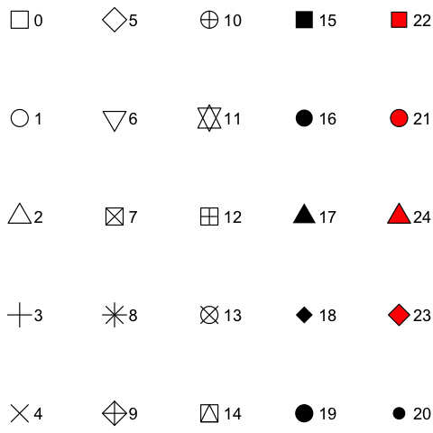
shape |
An
|
size |
A |
white_border |
Whether to include a white border around data points. Defaults to |
dodge_width |
For adjusting the distance between grouped objects. Defaults
to |
preserve |
Should dodging preserve the |
rasterize |
If |
rasterize_dpi |
The resolution in dots per inch (dpi) used for rastering
the layer if |
... |
Arguments passed on to the |
jitter_width |
Amount of random noise to be added to the
horizontal position of the of the data points. This can be useful to deal
with overplotting. Typical values range between |
jitter_height |
Amount of random noise to be added to the
vertical position of the of the data points. This can be useful to deal
with overplotting. Typical values range between |
cex |
Scaling for adjusting point spacing (see |
corral |
Method used to adjust points that would be placed too wide
horizontally. Options are |
corral.width |
Width of the corral, if not |
Details
-
add_data_points_beeswarm()is based onggbeeswarm::geom_beeswarm(). Check there for additional arguments. -
add_data_points()and friends support rasterization. See examples and Advanced plotting. -
add_data_points()and friends support data subsetting. See examples and Advanced plotting.
Value
A tidyplot object.
Examples
study |>
  tidyplot(x = treatment, y = score, color = treatment) |>
  add_data_points()

study |>
  tidyplot(x = treatment, y = score, color = treatment) |>
  add_data_points_jitter()

study |>
  tidyplot(x = treatment, y = score, color = treatment) |>
  add_data_points_beeswarm()

# Changing arguments
study |>
  tidyplot(x = treatment, y = score, color = treatment) |>
  add_data_points_jitter(jitter_width = 1)

animals |>
  tidyplot(x = weight, y = size) |>
  add_data_points(white_border = TRUE)

animals |>
  tidyplot(x = weight, y = size) |>
  add_data_points(alpha = 0.4)

# Rasterization
animals |>
  tidyplot(x = weight, y = size) |>
  add_data_points(rasterize = TRUE, rasterize_dpi = 50)

# Data subsetting
animals |>
  tidyplot(x = weight, y = size) |>
  add_data_points() |>
  add_data_points(data = filter_rows(size > 300), color = "red")
Add ellipse
Description
Add ellipse
Usage
add_ellipse(plot, ...)
Arguments
plot |
A |
... |
Arguments passed on to |
Value
A tidyplot object.
Examples
pca |>
  tidyplot(x = pc1, y = pc2, color = group) |>
  add_data_points() |>
  add_ellipse()

pca |>
  tidyplot(x = pc1, y = pc2, color = group) |>
  add_data_points() |>
  add_ellipse(level = 0.75)

pca |>
  tidyplot(x = pc1, y = pc2, color = group) |>
  add_data_points() |>
  add_ellipse(type = "norm")
Add heatmap
Description
Add heatmap
Usage
add_heatmap(
  plot,
  scale = c("none", "row", "column"),
  rotate_labels = 90,
  rasterize = FALSE,
  rasterize_dpi = 300,
  ...
)
Arguments
plot |
A |
scale |
Whether to compute row z scores for |
rotate_labels |
Degree to rotate the x-axis labels. Defaults to |
rasterize |
If |
rasterize_dpi |
The resolution in dots per inch (dpi) used for rastering
the layer if |
... |
Arguments passed on to the |
Details
-
add_heatmap()supports rasterization. See examples and Advanced plotting.
Value
A tidyplot object.
Examples
climate |>
  tidyplot(x = month, y = year, color = max_temperature) |>
  add_heatmap()

# Calculate row-wise z score
climate |>
  tidyplot(x = month, y = year, color = max_temperature) |>
  add_heatmap(scale = "row")

# Calculate column-wise z score
climate |>
  tidyplot(x = month, y = year, color = max_temperature) |>
  add_heatmap(scale = "column")

# Rasterize heatmap
climate |>
  tidyplot(x = month, y = year, color = max_temperature) |>
  add_heatmap(rasterize = TRUE, rasterize_dpi = 20)
Add histogram
Description
Add histogram
Usage
add_histogram(plot, binwidth = NULL, bins = NULL, ...)
Arguments
plot |
A |
binwidth |
The width of the bins. Can be specified as a numeric value
or as a function that takes x after scale transformation as input and
returns a single numeric value. When specifying a function along with a
grouping structure, the function will be called once per group.
The default is to use the number of bins in The bin width of a date variable is the number of days in each time; the bin width of a time variable is the number of seconds. |
bins |
Number of bins. Overridden by |
... |
Arguments passed on to the |
Value
A tidyplot object.
Examples
energy |>
  tidyplot(x = energy) |>
  add_histogram()

energy |>
  tidyplot(x = energy, color = energy_type) |>
  add_histogram()
Add line or area
Description
add_line() and add_area() connect individual data points, which is rarely needed.
In most cases, you are probably looking for add_sum_line(), add_mean_line(), add_sum_area() or add_mean_area().
Usage
add_line(
  plot,
  group,
  dodge_width = NULL,
  linewidth = 0.25,
  preserve = "total",
  ...
)

add_area(
  plot,
  group,
  dodge_width = NULL,
  linewidth = 0.25,
  alpha = 0.4,
  preserve = "total",
  ...
)
Arguments
plot |
A |
group |
Variable in the dataset to be used for grouping. |
dodge_width |
For adjusting the distance between grouped objects. Defaults
to |
linewidth |
Thickness of the line in points (pt). Typical values range between |
preserve |
Should dodging preserve the |
... |
Arguments passed on to the |
alpha |
A |
Value
A tidyplot object.
Examples
# Paired data points
study |>
  tidyplot(x = treatment, y = score, color = group) |>
  reorder_x_axis_labels("A", "C", "B", "D") |>
  add_data_points() |>
  add_line(group = participant, color = "grey")

study |>
  tidyplot(x = treatment, y = score) |>
  reorder_x_axis_labels("A", "C", "B", "D") |>
  add_data_points() |>
  add_area(group = participant)
Add mean
Description
Add mean
Usage
add_mean_bar(
  plot,
  dodge_width = NULL,
  width = 0.6,
  saturation = 1,
  preserve = "total",
  ...
)

add_mean_dash(
  plot,
  dodge_width = NULL,
  width = 0.6,
  linewidth = 0.25,
  preserve = "total",
  ...
)

add_mean_dot(plot, dodge_width = NULL, size = 2, preserve = "total", ...)

add_mean_value(
  plot,
  dodge_width = NULL,
  accuracy = 0.1,
  scale_cut = NULL,
  fontsize = 7,
  extra_padding = 0.15,
  vjust = NULL,
  hjust = NULL,
  preserve = "total",
  ...
)

add_mean_line(
  plot,
  group,
  dodge_width = NULL,
  linewidth = 0.25,
  preserve = "total",
  ...
)

add_mean_area(
  plot,
  group,
  dodge_width = NULL,
  linewidth = 0.25,
  preserve = "total",
  ...
)
Arguments
plot |
A |
dodge_width |
For adjusting the distance between grouped objects. Defaults
to |
width |
Horizontal width of the plotted object (bar, error bar, boxplot,
violin plot, etc). Typical values range between |
saturation |
A |
preserve |
Should dodging preserve the |
... |
Arguments passed on to the |
linewidth |
Thickness of the line in points (pt). Typical values range between |
size |
A |
accuracy |
A number to round to. Use (e.g.) Applied to rescaled data. |
scale_cut |
Scale cut function to be applied. See |
fontsize |
Font size in points. Defaults to |
extra_padding |
Extra padding to create space for the value label. |
vjust |
Vertical position adjustment of the value label. |
hjust |
Horizontal position adjustment of the value label. |
group |
Variable in the dataset to be used for grouping. |
Value
A tidyplot object.
Examples
study |>
  tidyplot(x = treatment, y = score, color = treatment) |>
  add_mean_bar()

study |>
  tidyplot(x = treatment, y = score, color = treatment) |>
  add_mean_dash()

study |>
  tidyplot(x = treatment, y = score, color = treatment) |>
  add_mean_dot()

study |>
  tidyplot(x = treatment, y = score, color = treatment) |>
  add_mean_value()

study |>
  tidyplot(x = treatment, y = score) |>
  add_mean_line()

study |>
  tidyplot(x = treatment, y = score) |>
  add_mean_area()

# Combination
study |>
  tidyplot(x = treatment, y = score) |>
  add_mean_bar(alpha = 0.4) |>
  add_mean_dash() |>
  add_mean_dot() |>
  add_mean_value() |>
  add_mean_line()

# Changing arguments: alpha
# Makes objects transparent
study |>
  tidyplot(x = treatment, y = score, color = treatment) |>
  theme_minimal_y() |>
  add_mean_bar(alpha = 0.4)

# Changing arguments: saturation
# Reduces fill color saturation without making the object transparent
study |>
  tidyplot(x = treatment, y = score, color = treatment) |>
  theme_minimal_y() |>
  add_mean_bar(saturation = 0.3)

# Changing arguments: accuracy
study |>
  tidyplot(x = treatment, y = score, color = treatment) |>
  add_mean_value(accuracy = 0.01)

# Changing arguments: fontsize
study |>
  tidyplot(x = treatment, y = score, color = treatment) |>
  add_mean_value(fontsize = 10)

# Changing arguments: color
study |>
  tidyplot(x = treatment, y = score, color = treatment) |>
  add_mean_value(color = "black")
Add median
Description
Add median
Usage
add_median_bar(
  plot,
  dodge_width = NULL,
  width = 0.6,
  saturation = 1,
  preserve = "total",
  ...
)

add_median_dash(
  plot,
  dodge_width = NULL,
  width = 0.6,
  linewidth = 0.25,
  preserve = "total",
  ...
)

add_median_dot(plot, dodge_width = NULL, size = 2, preserve = "total", ...)

add_median_value(
  plot,
  dodge_width = NULL,
  accuracy = 0.1,
  scale_cut = NULL,
  fontsize = 7,
  extra_padding = 0.15,
  vjust = NULL,
  hjust = NULL,
  preserve = "total",
  ...
)

add_median_line(
  plot,
  group,
  dodge_width = NULL,
  linewidth = 0.25,
  preserve = "total",
  ...
)

add_median_area(
  plot,
  group,
  dodge_width = NULL,
  linewidth = 0.25,
  preserve = "total",
  ...
)
Arguments
plot |
A |
dodge_width |
For adjusting the distance between grouped objects. Defaults
to |
width |
Horizontal width of the plotted object (bar, error bar, boxplot,
violin plot, etc). Typical values range between |
saturation |
A |
preserve |
Should dodging preserve the |
... |
Arguments passed on to the |
linewidth |
Thickness of the line in points (pt). Typical values range between |
size |
A |
accuracy |
A number to round to. Use (e.g.) Applied to rescaled data. |
scale_cut |
Scale cut function to be applied. See |
fontsize |
Font size in points. Defaults to |
extra_padding |
Extra padding to create space for the value label. |
vjust |
Vertical position adjustment of the value label. |
hjust |
Horizontal position adjustment of the value label. |
group |
Variable in the dataset to be used for grouping. |
Value
A tidyplot object.
Examples
study |>
  tidyplot(x = treatment, y = score, color = treatment) |>
  add_median_bar()

study |>
  tidyplot(x = treatment, y = score, color = treatment) |>
  add_median_dash()

study |>
  tidyplot(x = treatment, y = score, color = treatment) |>
  add_median_dot()

study |>
  tidyplot(x = treatment, y = score, color = treatment) |>
  add_median_value()

study |>
  tidyplot(x = treatment, y = score) |>
  add_median_line()

study |>
  tidyplot(x = treatment, y = score) |>
  add_median_area()

# Combination
study |>
  tidyplot(x = treatment, y = score) |>
  add_median_bar(alpha = 0.4) |>
  add_median_dash() |>
  add_median_dot() |>
  add_median_value() |>
  add_median_line()

# Changing arguments: alpha
# Makes objects transparent
study |>
  tidyplot(x = treatment, y = score, color = treatment) |>
  theme_minimal_y() |>
  add_median_bar(alpha = 0.4)

# Changing arguments: saturation
# Reduces fill color saturation without making the object transparent
study |>
  tidyplot(x = treatment, y = score, color = treatment) |>
  theme_minimal_y() |>
  add_median_bar(saturation = 0.3)

# Changing arguments: accuracy
study |>
  tidyplot(x = treatment, y = score, color = treatment) |>
  add_median_value(accuracy = 0.01)

# Changing arguments: fontsize
study |>
  tidyplot(x = treatment, y = score, color = treatment) |>
  add_median_value(fontsize = 10)

# Changing arguments: color
study |>
  tidyplot(x = treatment, y = score, color = treatment) |>
  add_median_value(color = "black")
Add pie or donut chart
Description
Add pie or donut chart
Usage
add_pie(plot, width = 1, reverse = FALSE, ...)

add_donut(plot, width = 1, reverse = FALSE, ...)
Arguments
plot |
A |
width |
Width of the donut ring. |
reverse |
Whether the order should be reversed or not. Defaults to |
... |
Arguments passed on to the |
Value
A tidyplot object.
Examples
# for a `count` only provide `color`
# `count` of the data points in each `energy_type` category
energy |>
  tidyplot(color = energy_type) |>
  add_pie()

energy |>
  tidyplot(color = energy_type) |>
  add_donut()

energy |>
  tidyplot(color = energy_type) |>
  add_donut(width = 0.5)

# for a `sum` provide `color` and `y`
# `sum` of `energy` in each `energy_type` category
energy |>
  tidyplot(y = energy, color = energy_type) |>
  add_pie()

energy |>
  tidyplot(y = energy, color = energy_type) |>
  add_donut()

energy |>
  tidyplot(y = energy, color = energy_type) |>
  add_donut(width = 0.5)
Add reference lines
Description
Add reference lines
Usage
add_reference_lines(
  plot,
  x = NULL,
  y = NULL,
  linetype = "dashed",
  linewidth = 0.25,
  ...
)
Arguments
plot |
A |
x |
Numeric values where the reference lines should meet the x-axis. For example, |
y |
Numeric values where the reference lines should meet the y-axis. For example, |
linetype |
Either an integer (0-6) or a name (0 = blank, 1 = solid, 2 = dashed, 3 = dotted, 4 = dotdash, 5 = longdash, 6 = twodash). |
linewidth |
Thickness of the line in points (pt). Typical values range between |
... |
Arguments passed on to the |
Value
A tidyplot object.
Examples
animals |>
  tidyplot(x = weight, y = speed) |>
   add_reference_lines(x = 4000, y = c(100, 200)) |>
   add_data_points()

animals |>
  tidyplot(x = weight, y = speed) |>
   add_reference_lines(x = 4000, y = c(100, 200), linetype = "dotdash") |>
   add_data_points()
Add error bar
Description
-
add_sem_errorbar()adds the standard error of mean. -
add_range_errorbar()adds the range from smallest to largest value. -
add_sd_errorbar()adds the standard deviation. -
add_ci95_errorbar()adds the 95% confidence interval.
Usage
add_sem_errorbar(
  plot,
  dodge_width = NULL,
  width = 0.4,
  linewidth = 0.25,
  preserve = "total",
  ...
)

add_range_errorbar(
  plot,
  dodge_width = NULL,
  width = 0.4,
  linewidth = 0.25,
  preserve = "total",
  ...
)

add_sd_errorbar(
  plot,
  dodge_width = NULL,
  width = 0.4,
  linewidth = 0.25,
  preserve = "total",
  ...
)

add_ci95_errorbar(
  plot,
  dodge_width = NULL,
  width = 0.4,
  linewidth = 0.25,
  preserve = "total",
  ...
)
Arguments
plot |
A |
dodge_width |
For adjusting the distance between grouped objects. Defaults
to |
width |
Width of the error bar. |
linewidth |
Thickness of the line in points (pt). Typical values range between |
preserve |
Should dodging preserve the |
... |
Arguments passed on to the |
Value
A tidyplot object.
Examples
# Standard error of the mean
study |>
  tidyplot(x = treatment, y = score, color = treatment) |>
  add_data_points() |>
  add_sem_errorbar()

# Range from minimum to maximum value
study |>
  tidyplot(x = treatment, y = score, color = treatment) |>
  add_data_points() |>
  add_range_errorbar()

# Standard deviation
study |>
  tidyplot(x = treatment, y = score, color = treatment) |>
  add_data_points() |>
  add_sd_errorbar()

# 95% confidence interval
study |>
  tidyplot(x = treatment, y = score, color = treatment) |>
  add_data_points() |>
  add_ci95_errorbar()

# Changing arguments: error bar width
study |>
  tidyplot(x = treatment, y = score, color = treatment) |>
  add_data_points() |>
  add_sem_errorbar(width = 0.8)

# Changing arguments: error bar line width
study |>
  tidyplot(x = treatment, y = score, color = treatment) |>
  add_data_points() |>
  add_sem_errorbar(linewidth = 1)
Add ribbon
Description
-
add_sem_ribbon()adds the standard error of mean. -
add_range_ribbon()adds the range from smallest to largest value. -
add_sd_ribbon()adds the standard deviation. -
add_ci95_ribbon()adds the 95% confidence interval.
Usage
add_sem_ribbon(plot, dodge_width = NULL, alpha = 0.4, color = NA, ...)

add_range_ribbon(plot, dodge_width = NULL, alpha = 0.4, color = NA, ...)

add_sd_ribbon(plot, dodge_width = NULL, alpha = 0.4, color = NA, ...)

add_ci95_ribbon(plot, dodge_width = NULL, alpha = 0.4, color = NA, ...)
Arguments
plot |
A |
dodge_width |
For adjusting the distance between grouped objects. Defaults
to |
alpha |
A |
color |
A hex color for the stroke color. For example, |
... |
Arguments passed on to the |
Value
A tidyplot object.
Examples
# Standard error of the mean
time_course |>
  tidyplot(x = day, y = score, color = treatment) |>
  add_mean_line() |>
  add_sem_ribbon()

# Range from minimum to maximum value
time_course |>
  tidyplot(x = day, y = score, color = treatment) |>
  add_mean_line() |>
  add_range_ribbon()

# Standard deviation
time_course |>
  tidyplot(x = day, y = score, color = treatment) |>
  add_mean_line() |>
  add_sd_ribbon()

# 95% confidence interval
time_course |>
  tidyplot(x = day, y = score, color = treatment) |>
  add_mean_line() |>
  add_ci95_ribbon()

# Changing arguments: alpha
time_course |>
  tidyplot(x = day, y = score, color = treatment) |>
  add_mean_line() |>
  add_sem_ribbon(alpha = 0.7)
Add sum
Description
Add sum
Usage
add_sum_bar(
  plot,
  dodge_width = NULL,
  width = 0.6,
  saturation = 1,
  preserve = "total",
  ...
)

add_sum_dash(
  plot,
  dodge_width = NULL,
  width = 0.6,
  linewidth = 0.25,
  preserve = "total",
  ...
)

add_sum_dot(plot, dodge_width = NULL, size = 2, preserve = "total", ...)

add_sum_value(
  plot,
  dodge_width = NULL,
  accuracy = 0.1,
  scale_cut = NULL,
  fontsize = 7,
  extra_padding = 0.15,
  vjust = NULL,
  hjust = NULL,
  preserve = "total",
  ...
)

add_sum_line(
  plot,
  group,
  dodge_width = NULL,
  linewidth = 0.25,
  preserve = "total",
  ...
)

add_sum_area(
  plot,
  group,
  dodge_width = NULL,
  linewidth = 0.25,
  preserve = "total",
  ...
)
Arguments
plot |
A |
dodge_width |
For adjusting the distance between grouped objects. Defaults
to |
width |
Horizontal width of the plotted object (bar, error bar, boxplot,
violin plot, etc). Typical values range between |
saturation |
A |
preserve |
Should dodging preserve the |
... |
Arguments passed on to the |
linewidth |
Thickness of the line in points (pt). Typical values range between |
size |
A |
accuracy |
A number to round to. Use (e.g.) Applied to rescaled data. |
scale_cut |
Scale cut function to be applied. See |
fontsize |
Font size in points. Defaults to |
extra_padding |
Extra padding to create space for the value label. |
vjust |
Vertical position adjustment of the value label. |
hjust |
Horizontal position adjustment of the value label. |
group |
Variable in the dataset to be used for grouping. |
Value
A tidyplot object.
Examples
spendings |>
  tidyplot(x = category, y = amount, color = category) |>
  adjust_x_axis(rotate_labels = TRUE) |>
  add_sum_bar()

spendings |>
  tidyplot(x = category, y = amount, color = category) |>
  adjust_x_axis(rotate_labels = TRUE) |>
  add_sum_dash()

spendings |>
  tidyplot(x = category, y = amount, color = category) |>
  adjust_x_axis(rotate_labels = TRUE) |>
  add_sum_dot()

spendings |>
  tidyplot(x = category, y = amount, color = category) |>
  adjust_x_axis(rotate_labels = TRUE) |>
  add_sum_value()

spendings |>
  tidyplot(x = category, y = amount) |>
  adjust_x_axis(rotate_labels = TRUE) |>
  add_sum_line()

spendings |>
  tidyplot(x = category, y = amount) |>
  adjust_x_axis(rotate_labels = TRUE) |>
  add_sum_area()

# Combination
spendings |>
  tidyplot(x = category, y = amount) |>
  adjust_x_axis(rotate_labels = TRUE) |>
  add_median_bar(alpha = 0.4) |>
  add_median_dash() |>
  add_median_dot() |>
  add_median_value() |>
  add_median_line()

# Changing arguments: alpha
# Makes objects transparent
spendings |>
  tidyplot(x = category, y = amount, color = category) |>
  theme_minimal_y() |>
  adjust_x_axis(rotate_labels = TRUE) |>
  add_sum_bar(alpha = 0.4)

# Changing arguments: saturation
# Reduces fill color saturation without making the object transparent
spendings |>
  tidyplot(x = category, y = amount, color = category) |>
  theme_minimal_y() |>
  adjust_x_axis(rotate_labels = TRUE) |>
  add_sum_bar(saturation = 0.3)

# Changing arguments: accuracy
spendings |>
  tidyplot(x = category, y = amount, color = category) |>
  adjust_x_axis(rotate_labels = TRUE) |>
  add_sum_value(accuracy = 1)

# Changing arguments: fontsize
spendings |>
  tidyplot(x = category, y = amount, color = category) |>
  adjust_x_axis(rotate_labels = TRUE) |>
  add_sum_value(fontsize = 10)

# Changing arguments: color
spendings |>
  tidyplot(x = category, y = amount, color = category) |>
  adjust_x_axis(rotate_labels = TRUE) |>
  add_sum_value(color = "black")

# Changing arguments: extra_padding
spendings |>
  tidyplot(x = category, y = amount, color = category) |>
  adjust_x_axis(rotate_labels = TRUE) |>
  add_sum_value(extra_padding = 0.5)
Add statistical test
Description
Add statistical test
Usage
add_test_pvalue(
  plot,
  padding_top = 0.15,
  method = "t_test",
  p.adjust.method = "none",
  ref.group = NULL,
  comparisons = NULL,
  paired_by = NULL,
  label = "{format_p_value(p.adj, 0.0001)}",
  label.size = 7/ggplot2::.pt,
  step.increase = 0.15,
  vjust = -0.25,
  bracket.nudge.y = 0.1,
  hide.ns = FALSE,
  p.adjust.by = "panel",
  symnum.args = list(cutpoints = c(0, 0.001, 0.01, 0.05, Inf), symbols = c("***", "**",
    "*", "ns")),
  color = plot$tidyplot$ink,
  hide_info = FALSE,
  ...
)

add_test_asterisks(
  plot,
  padding_top = 0.1,
  method = "t_test",
  p.adjust.method = "none",
  ref.group = NULL,
  comparisons = NULL,
  paired_by = NULL,
  label = "p.adj.signif",
  label.size = 10/ggplot2::.pt,
  step.increase = 0.2,
  vjust = 0.3,
  bracket.nudge.y = 0.15,
  hide.ns = TRUE,
  p.adjust.by = "panel",
  symnum.args = list(cutpoints = c(0, 0.001, 0.01, 0.05, Inf), symbols = c("***", "**",
    "*", "ns")),
  color = plot$tidyplot$ink,
  hide_info = FALSE,
  ...
)
Arguments
plot |
A |
padding_top |
Extra padding above the data points to accommodate the statistical comparisons. |
method |
a character string indicating which method to be used for
pairwise comparisons. Default is |
p.adjust.method |
method for adjusting p values (see
|
ref.group |
a character string or a numeric value specifying the reference group. If specified, for a given grouping variable, each of the group levels will be compared to the reference group (i.e. control group).
Allowed values can be:
|
comparisons |
A list of length-2 vectors. The entries in the vector are 2 integers that correspond to the index of the groups of interest, to be compared. |
paired_by |
Variable to be used for paired analysis. |
label |
character string specifying label. Can be:
. |
label.size |
change the size of the label text |
step.increase |
numeric vector with the increase in fraction of total height for every additional comparison to minimize overlap. |
vjust |
move the text up or down relative to the bracket. |
bracket.nudge.y |
Vertical adjustment to nudge brackets by (in fraction of the total height). Useful to move up or move down the bracket. If positive value, brackets will be moved up; if negative value, brackets are moved down. |
hide.ns |
can be logical value ( |
p.adjust.by |
possible value is one of |
symnum.args |
a list of arguments to pass to the function
In other words, we use the following convention for symbols indicating statistical significance:
|
color |
A hex color for the stroke color. For example, |
hide_info |
Whether to hide details about the statistical testing as caption. Defaults to |
... |
Arguments passed on to |
Details
-
add_test_pvalue()andadd_test_asterisks()useggpubr::geom_pwc(). Check there for additional arguments. Known limitation:
add_test_pvalue()andadd_test_asterisks()expect a discrete variable on the x-axis and a continuous variable on the y-axis. To produce horizontal plots, useflip_plot().
Value
A tidyplot object.
Examples
# Add p value
study |>
  tidyplot(x = dose, y = score, color = group) |>
  add_mean_dash() |>
  add_sem_errorbar() |>
  add_data_points() |>
  add_test_pvalue()

# Add asterisks
study |>
  tidyplot(x = dose, y = score, color = group) |>
  add_mean_dash() |>
  add_sem_errorbar() |>
  add_data_points() |>
  add_test_asterisks()

# Change stat method
study |>
  tidyplot(x = dose, y = score, color = group) |>
  add_mean_dash() |>
  add_sem_errorbar() |>
  add_data_points() |>
  add_test_pvalue(method = "wilcoxon")

# Change p.adjust method
study |>
  tidyplot(x = dose, y = score, color = group) |>
  add_mean_dash() |>
  add_sem_errorbar() |>
  add_data_points() |>
  add_test_pvalue(p.adjust.method = "bonferroni")

# Define reference group to test against
study |>
  tidyplot(x = treatment, y = score, color = treatment) |>
  add_mean_dash() |>
  add_sem_errorbar() |>
  add_data_points() |>
  add_test_asterisks(ref.group = 1)

# Define selected comparisons
study |>
  tidyplot(x = treatment, y = score, color = treatment) |>
  add_mean_dash() |>
  add_sem_errorbar() |>
  add_data_points() |>
  add_test_pvalue(comparisons = list(c(1,3),c(2,4)))

# Paired analysis
x <- c(2.3, 4.5, 6.3, 3.4, 7.8, 6.7)
df <- data.frame(
  x = c(x, x + c(0.8, 0.75)),
  group = paste0("g", rep(c(1, 2), each = 6)),
  batch = paste0("b", c(1:6, 1:6)),
  shuffle = paste0("c", c(1:6, 6:1))
)

df |>
  tidyplot(group, x, color = group) |>
  add_boxplot() |>
  add_data_points() |>
  add_test_pvalue(paired_by = shuffle) |>
  add_line(group = shuffle, color = "black")

df |>
  tidyplot(group, x, color = group) |>
  add_boxplot() |>
  add_data_points() |>
  add_test_pvalue(paired_by = batch) |>
  add_line(group = batch, color = "black")

# hide non-significant p values
gene_expression |>
  # filter to one gene
  dplyr::filter(external_gene_name == "Apol6") |>
  # start plotting
  tidyplot(x = condition, y = expression, color = sample_type) |>
  add_mean_dash() |>
  add_sem_errorbar() |>
  add_data_points() |>
  add_test_pvalue(hide.ns = TRUE)

# Flip plot
study |>
  tidyplot(x = treatment, y = score, color = treatment) |>
  add_mean_dash() |>
  add_sem_errorbar() |>
  add_data_points() |>
  add_test_asterisks(comparisons = list(c(1,4),c(2,3))) |>
  flip_plot()

# Adjust top padding for statistical comparisons
study |>
  tidyplot(x = treatment, y = score, color = treatment) |>
  add_mean_dash() |>
  add_sem_errorbar() |>
  add_data_points() |>
  add_test_pvalue(padding_top = 0.08)

# Hide stats information
study |>
  tidyplot(x = dose, y = score, color = group) |>
  add_mean_dash() |>
  add_sem_errorbar() |>
  add_data_points() |>
  add_test_pvalue(hide_info = TRUE)
Add plot title or caption
Description
Add plot title or caption
Usage
add_title(plot, title = ggplot2::waiver())

add_caption(plot, caption = ggplot2::waiver())
Arguments
plot |
A |
title |
Title of the plot. |
caption |
Caption of the plot. |
Details
-
add_title()andadd_caption()support plotmath expressions to include special characters. See examples and Advanced plotting.
Value
A tidyplot object.
Examples
study |>
  tidyplot(x = treatment, y = score) |>
  add_data_points_beeswarm() |>
  add_title("This is my title")

study |>
  tidyplot(x = treatment, y = score) |>
  add_data_points_beeswarm() |>
  add_caption("This is the fine print in the caption")

# Plotmath expression
study |>
  tidyplot(x = treatment, y = score) |>
  add_data_points_beeswarm() |>
  add_title("$H[2]*O~and~E==m*c^{2}$")
Add violin plot
Description
Add violin plot
Usage
add_violin(
  plot,
  dodge_width = NULL,
  alpha = 0.3,
  saturation = 1,
  trim = TRUE,
  linewidth = 0.25,
  scale = "width",
  ...
)
Arguments
plot |
A |
dodge_width |
For adjusting the distance between grouped objects. Defaults
to |
alpha |
A |
saturation |
A |
trim |
If |
linewidth |
Thickness of the line in points (pt). Typical values range between |
scale |
if "area" (default), all violins have the same area (before trimming the tails). If "count", areas are scaled proportionally to the number of observations. If "width", all violins have the same maximum width. |
... |
Arguments passed on to the |
Value
A tidyplot object.
Examples
study |>
  tidyplot(x = treatment, y = score, color = treatment) |>
  add_violin()

# Changing arguments:
study |>
  tidyplot(x = treatment, y = score, color = treatment) |>
  add_violin(saturation = 0.6)

study |>
  tidyplot(x = treatment, y = score, color = treatment) |>
  add_violin(draw_quantiles = c(0.25, 0.5, 0.75))

study |>
  tidyplot(x = treatment, y = score, color = treatment) |>
  add_violin(trim = FALSE)

study |>
  tidyplot(x = treatment, y = score, color = treatment) |>
  add_violin(linewidth = 1)
Adjust colors
Description
Adjust colors
Usage
adjust_colors(
  plot,
  new_colors = NULL,
  saturation = 1,
  labels = tidyplot_parse_labels(),
  downsample = c("evenly", "first", "last", "middle"),
  ...
)
Arguments
plot |
A |
new_colors |
A character vector of new hex colors to use. Can be a named character vector of hex colors to assign certain data labels to specific colors. |
saturation |
A |
labels |
One of the options below. Please note that when
|
downsample |
If too many colors are provided, whether to downsample |
... |
Arguments passed on to the ggplot2 |
Value
A tidyplot object.
See Also
colors_discrete_friendly(), colors_continuous_viridis(), colors_diverging_blue2brown(), and new_color_scheme()
Examples
# Plot without adjustments
study |>
  tidyplot(x = treatment, y = score, color = treatment) |>
  add_data_points() |>
  add_mean_bar(alpha = 0.4) |>
  add_sem_errorbar()

# Provide hex colors
study |>
  tidyplot(x = treatment, y = score, color = treatment) |>
  add_data_points() |>
  add_mean_bar(alpha = 0.4) |>
  add_sem_errorbar() |>
  adjust_colors(new_colors = c("#644296","#F08533","#3B78B0", "#D1352C"))

# Provide discrete color scheme
study |>
  tidyplot(x = treatment, y = score, color = treatment) |>
  add_data_points() |>
  add_mean_bar(alpha = 0.4) |>
  add_sem_errorbar() |>
  adjust_colors(new_colors = colors_discrete_seaside)

# Provide named vector
study |>
  tidyplot(x = treatment, y = score, color = treatment) |>
  add_data_points() |>
  add_mean_bar(alpha = 0.4) |>
  add_sem_errorbar() |>
  adjust_colors(new_colors = c(
    "A" = "pink",
    "B" = "purple",
    "C" = "grey",
    "D" = "blue"))

# Provide continuous color scheme
climate |>
  tidyplot(x = month, y = year, color = max_temperature) |>
  add_heatmap() |>
  adjust_colors(new_colors = colors_continuous_turbo)
Adjust font
Description
Adjust font
Usage
adjust_font(plot, fontsize = 7, family = NULL, face = NULL)
Arguments
plot |
A |
fontsize |
Font size in points. Defaults to |
family |
The typeface to use. The validity of this value will depend on
the graphics device being used for rendering the plot. See
the systemfonts vignette
for guidance on the best way to access fonts installed on your computer.
The values |
face |
Font face ("plain", "italic", "bold", "bold.italic") |
Value
A tidyplot object.
Examples
# Plot without adjustments
study |>
  tidyplot(x = treatment, y = score, color = treatment) |>
  add_data_points_beeswarm() |>
  add_mean_bar(alpha = 0.4) |>
  add_sem_errorbar()

# Increase font size
study |>
  tidyplot(x = treatment, y = score, color = treatment) |>
  add_data_points_beeswarm() |>
  add_mean_bar(alpha = 0.4) |>
  add_sem_errorbar() |>
  adjust_font(fontsize = 16)

# Change font family
study |>
  tidyplot(x = treatment, y = score, color = treatment) |>
  add_data_points_beeswarm() |>
  add_mean_bar(alpha = 0.4) |>
  add_sem_errorbar() |>
  adjust_font(family = "mono")

# Change font face
study |>
  tidyplot(x = treatment, y = score, color = treatment) |>
  add_data_points_beeswarm() |>
  add_mean_bar(alpha = 0.4) |>
  add_sem_errorbar() |>
  adjust_font(face = "bold")
Adjust legend
Description
Adjust legend
Usage
adjust_legend_title(
  plot,
  title = ggplot2::waiver(),
  fontsize = NULL,
  family = NULL,
  face = NULL,
  color = NULL,
  ...
)

adjust_legend_position(plot, position = "right")
Arguments
plot |
A |
title |
Legend title. |
fontsize |
Font size in points. Defaults to |
family |
The typeface to use. The validity of this value will depend on
the graphics device being used for rendering the plot. See
the systemfonts vignette
for guidance on the best way to access fonts installed on your computer.
The values |
face |
Font face ("plain", "italic", "bold", "bold.italic") |
color |
A hex color for the stroke color. For example, |
... |
Arguments passed on to |
position |
The position of the legend. Can be one of
|
Details
The
titleargument ofadjust_legend_title()supports plotmath expressions to include special characters. See examples and Advanced plotting.
Value
A tidyplot object.
Examples
# Plot without adjustments
study |>
  tidyplot(x = treatment, y = score, color = treatment) |>
  add_data_points_beeswarm() |>
  add_mean_bar(alpha = 0.4) |>
  add_sem_errorbar()

# New title
study |>
  tidyplot(x = treatment, y = score, color = treatment) |>
  add_data_points_beeswarm() |>
  add_mean_bar(alpha = 0.4) |>
  add_sem_errorbar() |>
  adjust_legend_title("My new legend title")

# New title with plotmath expression
study |>
  tidyplot(x = treatment, y = score, color = treatment) |>
  add_data_points_beeswarm() |>
  add_mean_bar(alpha = 0.4) |>
  add_sem_errorbar() |>
  adjust_legend_title("$E==m*c^{2}$")

# Alternative legend positions
study |>
  tidyplot(x = treatment, y = score, color = treatment) |>
  add_data_points_beeswarm() |>
  add_mean_bar(alpha = 0.4) |>
  add_sem_errorbar() |>
  adjust_legend_position("left")

study |>
  tidyplot(x = treatment, y = score, color = treatment) |>
  add_data_points_beeswarm() |>
  add_mean_bar(alpha = 0.4) |>
  add_sem_errorbar() |>
  adjust_legend_position("top")

study |>
  tidyplot(x = treatment, y = score, color = treatment) |>
  add_data_points_beeswarm() |>
  add_mean_bar(alpha = 0.4) |>
  add_sem_errorbar() |>
  adjust_legend_position("bottom")

# `position = "none"` hides the legend
study |>
  tidyplot(x = treatment, y = score, color = treatment) |>
  add_data_points_beeswarm() |>
  add_mean_bar(alpha = 0.4) |>
  add_sem_errorbar() |>
  adjust_legend_position("none")
Adjust plot area padding
Description
Adjust plot area padding
Usage
adjust_padding(
  plot,
  top = NA,
  right = NA,
  bottom = NA,
  left = NA,
  all = NA,
  force_continuous = FALSE,
  ...
)
Arguments
plot |
A |
top |
Extra space between the data points and the top. Defaults to |
right |
Extra space between the data points and the right. Defaults to |
bottom |
Extra space between the data points and the bottom. Defaults to |
left |
Extra space between the data points and the left. Defaults to |
all |
Extra space around the data pointst. Overwrites |
force_continuous |
Whether to force the axis to be continuous. Defaults to |
... |
Arguments passed on to the |
Value
A tidyplot object.
Examples
# Plot without adjustments
animals |>
  tidyplot(x = weight, y = size, color = family) |>
  add_data_points() |>
  adjust_padding()

# Increase plot area padding
animals |>
  tidyplot(x = weight, y = size, color = family) |>
  add_data_points() |>
  adjust_padding(all = 0.2)

animals |>
  tidyplot(x = weight, y = size, color = family) |>
  add_data_points() |>
  adjust_padding(top = 0.8)

animals |>
  tidyplot(x = weight, y = size, color = family) |>
  add_data_points() |>
  adjust_padding(bottom = 0.8)

animals |>
  tidyplot(x = weight, y = size, color = family) |>
  add_data_points() |>
  adjust_padding(right = 0.8)

animals |>
  tidyplot(x = weight, y = size, color = family) |>
  add_data_points() |>
  adjust_padding(left = 0.8)
Adjust plot area size
Description
Adjust plot area size
Usage
adjust_size(
  plot,
  width = NULL,
  height = NULL,
  unit = NULL,
  overall_width = NULL,
  overall_height = NULL
)
Arguments
plot |
A |
width, height |
Dimensions of the plot area. The default ( |
unit |
Unit of the plot area width and height. The default ( |
overall_width, overall_height |
The overall dimensions of a multiplot layout generated with |
Value
A tidyplot object.
Examples
# Plot without adjustments
study |>
  tidyplot(x = treatment, y = score, color = treatment) |>
  add_data_points_beeswarm(shape = 1) |>
  add_mean_bar(alpha = 0.4) |>
  add_sem_errorbar()

# Resize to 15 x 15 mm
study |>
  tidyplot(x = treatment, y = score, color = treatment) |>
  add_data_points_beeswarm(shape = 1) |>
  add_mean_bar(alpha = 0.4) |>
  add_sem_errorbar() |>
  adjust_size(width = 15, height = 15)

# Resize to 4 x 4 cm
study |>
  tidyplot(x = treatment, y = score, color = treatment) |>
  add_data_points_beeswarm(shape = 1) |>
  add_mean_bar(alpha = 0.4) |>
  add_sem_errorbar() |>
  adjust_size(width = 4, height = 4, unit = "cm")

# Remove absolute dimensions and take all available space.
# This is the ggplot2 default.
study |>
  tidyplot(x = treatment, y = score, color = treatment) |>
  add_data_points_beeswarm(shape = 1) |>
  add_mean_bar(alpha = 0.4) |>
  add_sem_errorbar() |>
  adjust_size(width = NA, height = NA)
Adjust theme details
Description
This function is a wrapper around ggplot2::theme(). To use the required theme
helper functions ggplot2::element_blank(), ggplot2::element_rect(),
ggplot2::element_line(), and ggplot2::element_text() you need to either load
the ggplot2 package via library(ggplot2) or use the ggplot2:: prefix as shown above.
Usage
adjust_theme_details(plot, ...)
Arguments
plot |
A |
... |
Arguments passed on to the |
Value
A tidyplot object.
Examples
study |>
  tidyplot(x = treatment, y = score, color = treatment) |>
  add_data_points_beeswarm() |>
  add_mean_bar(alpha = 0.4) |>
  adjust_theme_details(plot.background = ggplot2::element_rect(fill = "#FFEBFF"))
Adjust titles and caption
Description
Adjust titles and caption
Usage
adjust_title(
  plot,
  title = ggplot2::waiver(),
  fontsize = NULL,
  family = NULL,
  face = NULL,
  color = NULL,
  ...
)

adjust_x_axis_title(
  plot,
  title = ggplot2::waiver(),
  fontsize = NULL,
  family = NULL,
  face = NULL,
  color = NULL,
  ...
)

adjust_y_axis_title(
  plot,
  title = ggplot2::waiver(),
  fontsize = NULL,
  family = NULL,
  face = NULL,
  color = NULL,
  ...
)

adjust_caption(
  plot,
  caption = ggplot2::waiver(),
  fontsize = NULL,
  family = NULL,
  face = NULL,
  color = NULL,
  ...
)
Arguments
plot |
A |
title |
Plot or axes title. |
fontsize |
Font size in points. Defaults to |
family |
The typeface to use. The validity of this value will depend on
the graphics device being used for rendering the plot. See
the systemfonts vignette
for guidance on the best way to access fonts installed on your computer.
The values |
face |
Font face ("plain", "italic", "bold", "bold.italic") |
color |
A hex color for the stroke color. For example, |
... |
Arguments passed on to |
caption |
Plot caption. |
Details
Adjust the plot title, axis titles and caption
All functions support plotmath expressions to include special characters. See examples and Advanced plotting.
Value
A tidyplot object.
Examples
# Plot without adjustments
study |>
  tidyplot(x = treatment, y = score, color = treatment) |>
  add_data_points() |>
  add_mean_bar(alpha = 0.4) |>
  add_sem_errorbar()

# Adjust description
study |>
  tidyplot(x = treatment, y = score, color = treatment) |>
  add_data_points() |>
  add_mean_bar(alpha = 0.4) |>
  add_sem_errorbar() |>
  adjust_title("This is my fantastic plot title") |>
  adjust_x_axis_title("Treatment group") |>
  adjust_y_axis_title("Disease score") |>
  adjust_legend_title("Legend title") |>
  adjust_caption("Here goes the caption")

# Plotmath expressions
study |>
  tidyplot(x = treatment, y = score, color = treatment) |>
  add_data_points() |>
  add_mean_bar(alpha = 0.4) |>
  add_sem_errorbar() |>
  adjust_title("$H[2]*O$") |>
  adjust_x_axis_title("$H[2]*O$") |>
  adjust_y_axis_title("$H[2]*O$") |>
  adjust_legend_title("$H[2]*O$") |>
  adjust_caption("$H[2]*O$")
Adjust axes
Description
Adjust axes
Usage
adjust_x_axis(
  plot,
  title = ggplot2::waiver(),
  breaks = ggplot2::waiver(),
  labels = NULL,
  limits = NULL,
  padding = c(NA, NA),
  rotate_labels = FALSE,
  transform = "identity",
  cut_short_scale = FALSE,
  force_continuous = FALSE,
  ...
)

adjust_y_axis(
  plot,
  title = ggplot2::waiver(),
  breaks = ggplot2::waiver(),
  labels = NULL,
  limits = NULL,
  padding = c(NA, NA),
  rotate_labels = FALSE,
  transform = "identity",
  cut_short_scale = FALSE,
  force_continuous = FALSE,
  ...
)
Arguments
plot |
A |
title |
Axis title. |
breaks |
One of:
|
labels |
One of the options below. Please note that when
|
limits |
Axis limits. For example, with |
padding |
Extra space between the data points and the axes. Defaults to |
rotate_labels |
Whether to rotate axis labels. If |
transform |
For continuous scales, the name of a transformation object or the object itself. Built-in transformations include "asn", "atanh", "boxcox", "date", "exp", "hms", "identity", "log", "log10", "log1p", "log2", "logit", "modulus", "probability", "probit", "pseudo_log", "reciprocal", "reverse", "sqrt" and "time". A transformation object bundles together a transform, its inverse,
and methods for generating breaks and labels. Transformation objects
are defined in the scales package, and are called |
cut_short_scale |
Whether to shorten axis labels using |
force_continuous |
Whether to force the axis to be continuous. Defaults to |
... |
Arguments passed on to ggplot2 |
Details
The
titleargument ofadjust_x_axis()andadjust_y_axis()supports plotmath expressions to include special characters. See examples and Advanced plotting.
Value
A tidyplot object.
Examples
# Plot without adjustments
animals |>
  tidyplot(x = weight, y = size, color = family) |>
  add_data_points()

# New titles
animals |>
  tidyplot(x = weight, y = size, color = family) |>
  add_data_points() |>
  adjust_x_axis(title = "My new x-axis title") |>
  adjust_y_axis(title = "My new y-axis title")

# New titles with plotmath expressions
animals |>
  tidyplot(x = weight, y = size, color = family) |>
  add_data_points() |>
  adjust_x_axis(title = "$H[2]*O$") |>
  adjust_y_axis(title = "$E==m*c^{2}$")

# Axes limits
animals |>
  tidyplot(x = weight, y = size, color = family) |>
  add_data_points() |>
  adjust_x_axis(limits = c(-1000, 4000)) |>
  adjust_y_axis(limits = c(-200, 600))

# Rotate labels
animals |>
  tidyplot(x = weight, y = size, color = family) |>
  add_data_points() |>
  adjust_x_axis(rotate_labels = 90) |>
  adjust_y_axis(rotate_labels = 90)

# Increase plot area padding
animals |>
  tidyplot(x = weight, y = size, color = family) |>
  add_data_points() |>
  adjust_x_axis(padding = c(0.2, 0.2)) |>
  adjust_y_axis(padding = c(0.2, 0.2))

# Scale transformation
animals |>
  tidyplot(x = weight, y = size, color = family) |>
  add_data_points() |>
  adjust_x_axis(transform = "log10") |>
  adjust_y_axis(transform = "log2")
Subset data rows
Description
Subset data rows
Usage
all_rows()

filter_rows(..., .by = NULL)

max_rows(order_by, n, by = NULL, with_ties = TRUE, na_rm = FALSE)

min_rows(order_by, n, by = NULL, with_ties = TRUE, na_rm = FALSE)

first_rows(n, by = NULL)

last_rows(n, by = NULL)

sample_rows(n, by = NULL)
Arguments
... |
< |
.by, by |
< |
order_by |
< |
n |
The number of rows to select. If not are supplied, A negative value of |
with_ties |
Should ties be kept together? The default, |
na_rm |
Should missing values in |
![[Experimental]](./figures/lifecycle-experimental.svg)
Value
A function to achieve the desired data subsetting.
Examples
# Highlight all animals
animals |>
 tidyplot(x = weight, y = size) |>
 add_data_points() |>
 add_data_points(data = all_rows(),
  color = "red", shape = 1, size = 3)

# Highlight 3 animals with the highest weight
animals |>
 tidyplot(x = weight, y = size) |>
 add_data_points() |>
 add_data_points(data = max_rows(weight, n = 3),
  color = "red", shape = 1, size = 3)

# Highlight 3 animals with the lowest weight
animals |>
 tidyplot(x = weight, y = size) |>
 add_data_points() |>
 add_data_points(data = min_rows(weight, n = 3),
  color = "red", shape = 1, size = 3)

# Highlight the first 3 animals in the dataset
animals |>
 tidyplot(x = weight, y = size) |>
 add_data_points() |>
 add_data_points(data = first_rows(n = 3),
  color = "red", shape = 1, size = 3)

# Highlight the last 3 animals in the dataset
animals |>
 tidyplot(x = weight, y = size) |>
 add_data_points() |>
 add_data_points(data = last_rows(n = 3),
  color = "red", shape = 1, size = 3)

# Highlight 3 random animals
animals |>
 tidyplot(x = weight, y = size) |>
 add_data_points() |>
 add_data_points(data = sample_rows(n = 3),
  color = "red", shape = 1, size = 3)
Animals data
Description
Animals data
Usage
animals
Format
A data frame.
Source
ChatGPT-3.5, Caution: The accuracy of the data has not been verified.
Examples
dplyr::glimpse(animals)
Climate data
Description
Climate data
Usage
climate
Format
A data frame.
Source
National Oceanic and Atmospheric Administration, Temperature data, weather station Hamburg Fuhlsbüttel, Germany
Examples
dplyr::glimpse(climate)
Continuous color schemes
Description
For more information about the use of color schemes in tidyplots, check out this article: Color schemes
Usage
colors_continuous_viridis

colors_continuous_magma

colors_continuous_inferno

colors_continuous_plasma

colors_continuous_cividis

colors_continuous_rocket

colors_continuous_mako

colors_continuous_turbo

colors_continuous_bluepinkyellow
Format
An object of class tidycolor (inherits from character) of length 265.
An object of class tidycolor (inherits from character) of length 265.
An object of class tidycolor (inherits from character) of length 265.
An object of class tidycolor (inherits from character) of length 265.
An object of class tidycolor (inherits from character) of length 265.
An object of class tidycolor (inherits from character) of length 265.
An object of class tidycolor (inherits from character) of length 265.
An object of class tidycolor (inherits from character) of length 265.
An object of class tidycolor (inherits from character) of length 11.
Details
Color schemes can be conveniently previewed by using the print method of the
tidycolor class. This will send a html preview to the RStudio Viewer pane.
colors_continuous_viridis
colors_continuous_viridis
A tidyplots color scheme with 265 colors, downsampled to 42 colors.c(
"#440154FF","#460A5DFF","#471264FF","#481B6DFF","#482374FF","#472C7AFF","#46337FFF","#443A83FF","#424186FF","#3F4889FF","#3C508BFF","#39568CFF","#365D8DFF","#33638DFF","#306A8EFF","#2D708EFF","#2B758EFF","#297B8EFF","#26818EFF","#24878EFF","#228D8DFF","#20928CFF","#1F988BFF","#1F9F88FF","#20A486FF","#24AA83FF","#29AF7FFF","#31B57BFF","#3BBB75FF","#45C06FFF","#53C569FF","#5EC962FF","#6ECE58FF","#7BD250FF","#8AD647FF","#9CD93CFF","#AADC32FF","#BDDF26FF","#CCE11EFF","#DEE318FF","#EDE51BFF","#FDE725FF")
colors_continuous_magma
colors_continuous_magma
A tidyplots color scheme with 265 colors, downsampled to 42 colors.c(
"#000004FF","#02020DFF","#060519FF","#0C0927FF","#130D34FF","#1C1044FF","#231252FF","#2E1162FF","#38106CFF","#420F75FF","#4E117BFF","#57157EFF","#611880FF","#6A1C81FF","#752181FF","#7D2482FF","#882781FF","#922B81FF","#9B2E7FFF","#A6317DFF","#AF357BFF","#BB3978FF","#C43C75FF","#CF4070FF","#D8456CFF","#DF4B68FF","#E85362FF","#EE5B5EFF","#F4675CFF","#F7715CFF","#FA7E5EFF","#FC8961FF","#FD9668FF","#FEA16EFF","#FEAB75FF","#FEB87EFF","#FEC287FF","#FECF92FF","#FDD99BFF","#FDE6A8FF","#FCF0B2FF","#FCFDBFFF")
colors_continuous_inferno
colors_continuous_inferno
A tidyplots color scheme with 265 colors, downsampled to 42 colors.c(
"#000004FF","#02020EFF","#07051AFF","#0D082AFF","#150B37FF","#1F0C48FF","#290B54FF","#350A60FF","#3E0966FF","#490B6AFF","#540F6DFF","#5D126EFF","#68166EFF","#71196EFF","#7C1D6DFF","#85216BFF","#8F2568FF","#992766FF","#A22B62FF","#AD305DFF","#B53458FF","#C03952FF","#C73E4CFF","#D04545FF","#D84C3EFF","#DF5237FF","#E55C30FF","#EB6429FF","#F06F20FF","#F47918FF","#F7840FFF","#F98E09FF","#FB9B06FF","#FCA60CFF","#FCB115FF","#FBBF24FF","#F9C932FF","#F6D746FF","#F3E259FF","#F1EE73FF","#F3F68BFF","#FCFFA4FF")
colors_continuous_plasma
colors_continuous_plasma
A tidyplots color scheme with 265 colors, downsampled to 42 colors.c(
"#0D0887FF","#1C068EFF","#290593FF","#360498FF","#3F049CFF","#4B03A1FF","#5502A4FF","#5F01A6FF","#6700A8FF","#7100A8FF","#7B02A8FF","#8405A7FF","#8E0BA5FF","#9511A1FF","#9E199DFF","#A62098FF","#AD2792FF","#B42E8DFF","#BB3488FF","#C23C81FF","#C8437BFF","#CD4A76FF","#D35171FF","#D9586AFF","#DE5F65FF","#E26560FF","#E76E5BFF","#EB7556FF","#EF7E50FF","#F3854BFF","#F68E44FF","#F89540FF","#FB9F3AFF","#FCA835FF","#FDB030FF","#FEBA2CFF","#FDC328FF","#FCCE25FF","#FAD824FF","#F7E325FF","#F4ED27FF","#F0F921FF")
colors_continuous_cividis
colors_continuous_cividis
A tidyplots color scheme with 265 colors, downsampled to 42 colors.c(
"#00204DFF","#002557FF","#002961FF","#002D6DFF","#00306FFF","#01366EFF","#173A6DFF","#253E6CFF","#2E436CFF","#36476BFF","#3F4C6BFF","#45506BFF","#4C546CFF","#52596CFF","#595E6DFF","#5E626EFF","#64666FFF","#696B71FF","#6E6F73FF","#747475FF","#797977FF","#7F7D78FF","#848279FF","#8B8779FF","#918C78FF","#979178FF","#9D9677FF","#A39A76FF","#ABA074FF","#B1A573FF","#B7AA71FF","#BEAF6FFF","#C5B56CFF","#CCBB69FF","#D2C066FF","#D9C562FF","#E0CB5EFF","#E8D259FF","#EED753FF","#F7DD4DFF","#FDE346FF","#FFEA46FF")
colors_continuous_rocket
colors_continuous_rocket
A tidyplots color scheme with 265 colors, downsampled to 42 colors.c(
"#03051AFF","#0A091FFF","#120D25FF","#1C112BFF","#241432FF","#2E1739FF","#36193FFF","#411B44FF","#491D49FF","#531E4DFF","#5E1F52FF","#671F55FF","#721F57FF","#7B1F59FF","#871E5BFF","#921C5BFF","#9D1B5BFF","#A7195AFF","#B01759FF","#BC1656FF","#C51852FF","#CE1D4EFF","#D62449FF","#DE2E44FF","#E43841FF","#E8413EFF","#ED4F3EFF","#EF5A41FF","#F26747FF","#F3724EFF","#F47E57FF","#F58860FF","#F5946BFF","#F69D75FF","#F6A77FFF","#F6B28CFF","#F6BB97FF","#F7C6A6FF","#F7CEB2FF","#F8D8C1FF","#F9E0CEFF","#FAEBDDFF")
colors_continuous_mako
colors_continuous_mako
A tidyplots color scheme with 265 colors, downsampled to 42 colors.c(
"#0B0405FF","#12080DFF","#180D16FF","#1E111FFF","#241628FF","#2A1B33FF","#2F1F3DFF","#342547FF","#372852FF","#3B2D5BFF","#3E3367FF","#403871FF","#413E7EFF","#414387FF","#3F4B90FF","#3D5296FF","#3A5A9AFF","#38619DFF","#37689FFF","#3670A0FF","#3576A2FF","#357DA3FF","#3484A5FF","#348CA7FF","#3492A8FF","#3499AAFF","#35A0ABFF","#37A6ACFF","#3AAEADFF","#3FB5ADFF","#44BDADFF","#4BC2ADFF","#55CAADFF","#61CFACFF","#72D4ADFF","#86D9B1FF","#96DDB5FF","#A9E1BDFF","#B6E6C5FF","#C5EAD0FF","#D0EFDAFF","#DEF5E5FF")
colors_continuous_turbo
colors_continuous_turbo
A tidyplots color scheme with 265 colors, downsampled to 42 colors.c(
"#30123BFF","#372365FF","#3D3489FF","#4147AEFF","#4456C8FF","#4669E0FF","#4777EFFF","#4688FBFF","#4197FFFF","#38A5FBFF","#2CB7F0FF","#22C4E3FF","#1AD3D1FF","#18DDC2FF","#1DE7B2FF","#29EFA2FF","#3DF58CFF","#53FA79FF","#69FD66FF","#83FF51FF","#98FE43FF","#AAFB39FF","#BAF635FF","#CBED34FF","#D9E436FF","#E4DA38FF","#F0CC3AFF","#F7C13AFF","#FCB136FF","#FEA230FF","#FE8F28FF","#FB7D21FF","#F56918FF","#EF5911FF","#E74A0CFF","#DD3C08FF","#D23105FF","#C32503FF","#B51C01FF","#A31301FF","#910B01FF","#7A0403FF")
colors_continuous_bluepinkyellow
colors_continuous_bluepinkyellow
A tidyplots color scheme with 11 colors.c(
"#00034D","#000F9F","#001CEF","#241EF5","#5823F6","#A033E0","#E85AB1","#F1907C","#F4AF63","#FCE552","#FFFB6D")
Discrete color schemes
Description
For more information about the use of color schemes in tidyplots, check out this article: Color schemes
Usage
colors_discrete_friendly

colors_discrete_seaside

colors_discrete_apple

colors_discrete_friendly_long

colors_discrete_okabeito

colors_discrete_ibm

colors_discrete_metro

colors_discrete_candy

colors_discrete_alger

colors_discrete_rainbow
Format
An object of class tidycolor (inherits from character) of length 6.
An object of class tidycolor (inherits from character) of length 5.
An object of class tidycolor (inherits from character) of length 7.
An object of class tidycolor (inherits from character) of length 7.
An object of class tidycolor (inherits from character) of length 7.
An object of class tidycolor (inherits from character) of length 5.
An object of class tidycolor (inherits from character) of length 5.
An object of class tidycolor (inherits from character) of length 5.
An object of class tidycolor (inherits from character) of length 5.
An object of class tidycolor (inherits from character) of length 9.
Details
The signature theme of tidyplots colors_discrete_friendly was adapted from
the Okabe & Ito color palette that was designed
to work well for people with color vision deficiency.
Color schemes can be conveniently previewed by using the print method of the
tidycolor class. This will send a html preview to the RStudio Viewer pane.
colors_discrete_friendly
colors_discrete_friendly
A tidyplots color scheme with 6 colors.c(
"#0072B2","#56B4E9","#009E73","#F5C710","#E69F00","#D55E00")
colors_discrete_seaside
colors_discrete_seaside
A tidyplots color scheme with 5 colors.c(
"#8ecae6","#219ebc","#023047","#ffb703","#fb8500")
colors_discrete_apple
colors_discrete_apple
A tidyplots color scheme with 7 colors.c(
"#ff3b30","#ff9500","#ffcc00","#4cd964","#5ac8fa","#007aff","#5856d6")
colors_discrete_friendly_long
colors_discrete_friendly_long
A tidyplots color scheme with 7 colors.c(
"#CC79A7","#0072B2","#56B4E9","#009E73","#F5C710","#E69F00","#D55E00")
colors_discrete_okabeito
colors_discrete_okabeito
A tidyplots color scheme with 7 colors.c(
"#E69F00","#56B4E9","#009E73","#F0E442","#0072B2","#D55E00","#CC79A7")
colors_discrete_ibm
colors_discrete_ibm
A tidyplots color scheme with 5 colors.c(
"#5B8DFE","#725DEE","#DD227D","#FE5F00","#FFB109")
colors_discrete_metro
colors_discrete_metro
A tidyplots color scheme with 5 colors.c(
"#4DACD6","#4FAE62","#F6C54D","#E37D46","#C02D45")
colors_discrete_candy
colors_discrete_candy
A tidyplots color scheme with 5 colors.c(
"#9b5de5","#f15bb5","#fee440","#00bbf9","#00f5d4")
colors_discrete_alger
colors_discrete_alger
A tidyplots color scheme with 5 colors.c(
"#000000","#1A5B5B","#ACC8BE","#F4AB5C","#D1422F")
colors_discrete_rainbow
colors_discrete_rainbow
A tidyplots color scheme with 9 colors.c(
"#FF7777","#FFAB74","#FFE577","#DBF47B","#91E480","#7CC9E5","#7DA8E6","#887DE6","#BC7BE4")
Diverging color schemes
Description
For more information about the use of color schemes in tidyplots, check out this article: Color schemes
Usage
colors_diverging_blue2red

colors_diverging_blue2brown

colors_diverging_BuRd

colors_diverging_BuYlRd

colors_diverging_spectral

colors_diverging_icefire
Format
An object of class tidycolor (inherits from character) of length 17.
An object of class tidycolor (inherits from character) of length 17.
An object of class tidycolor (inherits from character) of length 11.
An object of class tidycolor (inherits from character) of length 11.
An object of class tidycolor (inherits from character) of length 96.
An object of class tidycolor (inherits from character) of length 96.
Details
Color schemes can be conveniently previewed by using the print method of the
tidycolor class. This will send a html preview to the RStudio Viewer pane.
colors_diverging_blue2red
colors_diverging_blue2red
A tidyplots color scheme with 17 colors.c(
"#0000FF","#1F1FFF","#3F3FFF","#5F5FFF","#7F7FFF","#9F9FFF","#BFBFFF","#DFDFFF","#FFFFFF","#FFDFDF","#FFBFBF","#FF9F9F","#FF7F7F","#FF5F5F","#FF3F3F","#FF1F1F","#FF0000")
colors_diverging_blue2brown
colors_diverging_blue2brown
A tidyplots color scheme with 17 colors.c(
"#1961A5","#2671B5","#2D80BF","#268CC9","#119DD8","#00B2EB","#66C5EF","#C4E5F8","#FEFCF6","#FDEEB8","#FCDD67","#F6C445","#E78B43","#DD5642","#DB3E34","#CA3632","#B3322E")
colors_diverging_BuRd
colors_diverging_BuRd
A tidyplots color scheme with 11 colors.c(
"#053061","#2166AC","#4393C3","#92C5DE","#D1E5F0","#F7F7F7","#FDDBC7","#F4A582","#D6604D","#B2182B","#67001F")
colors_diverging_BuYlRd
colors_diverging_BuYlRd
A tidyplots color scheme with 11 colors.c(
"#313695","#4575B4","#74ADD1","#ABD9E9","#E0F3F8","#FFFFBF","#FEE090","#FDAE61","#F46D43","#D73027","#A50026")
colors_diverging_spectral
colors_diverging_spectral
A tidyplots color scheme with 96 colors, downsampled to 42 colors.c(
"#5b53a4","#525fa9","#486cb0","#3f77b5","#3389bd","#3d95b8","#47a0b3","#58b2ac","#64c0a6","#71c6a5","#86cfa5","#94d4a4","#a2d9a4","#b5e1a2","#c3e79f","#cfec9d","#e1f399","#e9f69d","#eef8a4","#f6fbb0","#fcfeba","#fffdbc","#fff7b2","#feeda1","#fee797","#fee08b","#fed27f","#fdc776","#fdbd6d","#fdad60","#fba05b","#f99153","#f67f4b","#f47044","#ef6645","#e55749","#df4e4b","#d9444d","#cb334d","#be254a","#b41947","#a90d45")
colors_diverging_icefire
colors_diverging_icefire
A tidyplots color scheme with 96 colors, downsampled to 42 colors.c(
"#b7e3d9","#a9d9d6","#98cdd2","#8ac4d0","#72b6ce","#63adcd","#55a3cd","#4394ce","#3987cf","#377cd0","#3f69c9","#465ebe","#4954b0","#474792","#42407b","#3c3a69","#323050","#2c2b42","#272636","#212028","#1f1e21","#201e1e","#261e1f","#332023","#3d2228","#4a252e","#5c2935","#6d2b3b","#7b2d40","#932e44","#a22f44","#b33341","#c53c3c","#d24737","#da5334","#e66734","#eb753a","#ef8445","#f39a5f","#f7ab75","#fab887","#fcc69a")
Common arguments
Description
Common arguments
Arguments
plot |
A |
data |
The data to be displayed in this layer. There are three options:
|
dodge_width |
For adjusting the distance between grouped objects. Defaults
to |
preserve |
Should dodging preserve the |
rasterize |
If |
rasterize_dpi |
The resolution in dots per inch (dpi) used for rastering
the layer if |
shape |
An
|
size |
A |
width |
Horizontal width of the plotted object (bar, error bar, boxplot,
violin plot, etc). Typical values range between |
linewidth |
Thickness of the line in points (pt). Typical values range between |
... |
Arguments passed on to the |
alpha |
A |
color |
A hex color for the stroke color. For example, |
fill |
A hex color for the fill color. For example, |
saturation |
A |
group |
Variable in the dataset to be used for grouping. |
reverse |
Whether the order should be reversed or not. Defaults to |
.reverse |
Whether the order should be reversed or not. Defaults to |
scale_cut |
Scale cut function to be applied. See |
fontsize |
Font size in points. Defaults to |
replace_na |
Whether to replace |
force_continuous |
Whether to force the axis to be continuous. Defaults to |
jitter_width |
Amount of random noise to be added to the
horizontal position of the of the data points. This can be useful to deal
with overplotting. Typical values range between |
jitter_height |
Amount of random noise to be added to the
vertical position of the of the data points. This can be useful to deal
with overplotting. Typical values range between |
Value
A tidyplot object.
Dinosaurs data
Description
Dinosaurs data
Usage
dinosaurs
Format
A data frame.
Source
ChatGPT-3.5, Caution: The accuracy of the data has not been verified.
Examples
dplyr::glimpse(dinosaurs)
Distributions data
Description
Distributions data
Usage
distributions
Format
A data frame.
Source
tidyplots package
Examples
dplyr::glimpse(distributions)
Energy data
Description
Energy data
Usage
energy
Format
A data frame.
Source
Energy-Charts, Energy production data, Germany
Examples
dplyr::glimpse(energy)
Energy week data
Description
Energy week data
Usage
energy_week
Format
A data frame.
Source
Energy-Charts, Energy production data, Germany
Examples
dplyr::glimpse(energy_week)
EU countries data
Description
EU countries data
Usage
eu_countries
Format
A data frame.
Source
ChatGPT-3.5, Caution: The accuracy of the data has not been verified.
Examples
dplyr::glimpse(eu_countries)
Flip x and y-axis
Description
![[Superseded]](./figures/lifecycle-superseded.svg)
This function is superseded because in many cases, flip_plot() can easily
be replaced by swapping the x and y axis. Some plot components additionally
require to set the orientation argument to "y".
Usage
flip_plot(plot, ...)
Arguments
plot |
A |
... |
Arguments passed on to |
Value
A tidyplot object.
Examples
study |>
  tidyplot(x = treatment, y = score, color = treatment) |>
  add_data_points() |>
  add_mean_bar(alpha = 0.4) |>
  add_sem_errorbar() |>
  flip_plot()

energy |>
  tidyplot(x = year, y = energy, color = energy_type) |>
  add_barstack_absolute() |>
  flip_plot()

# Better solutions without `flip_plot()`
study |>
  tidyplot(x = score, y = treatment, color = treatment) |>
  add_data_points() |>
  add_mean_bar(alpha = 0.4) |>
  add_sem_errorbar()

energy |>
  tidyplot(x = energy, y = year, color = energy_type) |>
  add_barstack_absolute(orientation = "y")
Format p values
Description
Format p values
Usage
format_p_value(x, accuracy = 1e-04)
Arguments
x |
A |
accuracy |
A number to round to. For example, use |
Value
Formatted number as character string.
Examples
format_p_value(0.03445553)
format_p_value(0.0003445553)
format_p_value(0.00003445553)
RNA-Seq expression data
Description
RNA-Seq expression data
Usage
gene_expression
Format
A data frame.
Source
Bassoon proteinopathy drives neurodegeneration in multiple sclerosis, Nature Neuroscience 2019
GSE104899, Gene Expression Omnibus
Examples
dplyr::glimpse(gene_expression)
New color scheme
Description
For more information about the use of color schemes in tidyplots, check out this article: Color schemes
Usage
new_color_scheme(x, name = "Untitled color scheme", reverse = FALSE)
Arguments
x |
Character vector of hex colors. For example |
name |
Name of the custom color scheme. |
reverse |
Whether the order should be reversed or not. Defaults to |
Value
A tidyplot object.
Examples
new_color_scheme(c("#ECA669","#E06681","#8087E2","#E2D269"))

new_color_scheme(c("#ECA669","#E06681","#8087E2","#E2D269"),
  name = "my_custom_color_scheme")
Principle component analysis data
Description
Principle component analysis data
Usage
pca
Format
A data frame.
Source
Bassoon proteinopathy drives neurodegeneration in multiple sclerosis, Nature Neuroscience 2019
Examples
dplyr::glimpse(pca)
Remove legend or legend title
Description
Remove legend or legend title
Usage
remove_legend(plot)

remove_legend_title(plot)
Arguments
plot |
A |
Value
A tidyplot object.
Examples
# Before removing
study |>
  tidyplot(x = treatment, y = score, color = treatment) |>
  add_mean_bar()

# After removing
study |>
  tidyplot(x = treatment, y = score, color = treatment) |>
  add_mean_bar() |>
  remove_legend_title()

study |>
  tidyplot(x = treatment, y = score, color = treatment) |>
  add_mean_bar() |>
  remove_legend()
Remove plot area padding
Description
Remove plot area padding
Usage
remove_padding(plot, force_continuous = FALSE)
Arguments
plot |
A |
force_continuous |
Whether to force the axis to be continuous. Defaults to |
Value
A tidyplot object.
Examples
# Before removing
animals |>
  tidyplot(x = weight, y = speed, color = family) |>
  add_data_points()

# After removing
animals |>
  tidyplot(x = weight, y = speed, color = family) |>
  add_data_points() |>
  remove_padding()
Remove plot title or caption
Description
Remove plot title or caption
Usage
remove_title(plot)

remove_caption(plot)
Arguments
plot |
A |
Value
A tidyplot object.
Examples
# Before removing
animals |>
  tidyplot(x = weight, y = speed, color = family) |>
  add_data_points() |>
  add_title("Name of the plot") |>
  add_caption("This is the caption")

# After removing
animals |>
  tidyplot(x = weight, y = speed, color = family) |>
  add_data_points() |>
  add_title("Name of the plot") |>
  add_caption("This is the caption") |>
  remove_title()

animals |>
  tidyplot(x = weight, y = speed, color = family) |>
  add_data_points() |>
  add_title("Name of the plot") |>
  add_caption("This is the caption") |>
  remove_caption()
Remove x-axis or parts of it
Description
Remove x-axis or parts of it
Usage
remove_x_axis(plot)

remove_x_axis_line(plot)

remove_x_axis_ticks(plot)

remove_x_axis_labels(plot)

remove_x_axis_title(plot)
Arguments
plot |
A |
Value
A tidyplot object.
Examples
# Before removing
study |>
  tidyplot(x = treatment, y = score, color = treatment) |>
  add_mean_bar()

# After removing
study |>
  tidyplot(x = treatment, y = score, color = treatment) |>
  add_mean_bar() |>
  remove_x_axis_line()

study |>
  tidyplot(x = treatment, y = score, color = treatment) |>
  add_mean_bar() |>
  remove_x_axis_ticks()

study |>
  tidyplot(x = treatment, y = score, color = treatment) |>
  add_mean_bar() |>
  remove_x_axis_labels()

study |>
  tidyplot(x = treatment, y = score, color = treatment) |>
  add_mean_bar() |>
  remove_x_axis_title()

study |>
  tidyplot(x = treatment, y = score, color = treatment) |>
  add_mean_bar() |>
  remove_x_axis()
Remove y-axis or parts of it
Description
Remove y-axis or parts of it
Usage
remove_y_axis(plot)

remove_y_axis_line(plot)

remove_y_axis_ticks(plot)

remove_y_axis_labels(plot)

remove_y_axis_title(plot)
Arguments
plot |
A |
Value
A tidyplot object.
Examples
# Before removing
study |>
  tidyplot(x = treatment, y = score, color = treatment) |>
  add_mean_bar()

# After removing
study |>
  tidyplot(x = treatment, y = score, color = treatment) |>
  add_mean_bar() |>
  remove_y_axis_line()

study |>
  tidyplot(x = treatment, y = score, color = treatment) |>
  add_mean_bar() |>
  remove_y_axis_ticks()

study |>
  tidyplot(x = treatment, y = score, color = treatment) |>
  add_mean_bar() |>
  remove_y_axis_labels()

study |>
  tidyplot(x = treatment, y = score, color = treatment) |>
  add_mean_bar() |>
  remove_y_axis_title()

study |>
  tidyplot(x = treatment, y = score, color = treatment) |>
  add_mean_bar() |>
  remove_y_axis()
Rename axis or color levels
Description
Rename axis or color levels
Usage
rename_x_axis_levels(plot, new_names)

rename_y_axis_levels(plot, new_names)

rename_color_levels(plot, new_names)
Arguments
plot |
A |
new_names |
Named character vector in the format c("old1" = "new1", "old2" = "new2"). |
Value
A tidyplot object.
Examples
# Before adjustments
study |>
  tidyplot(x = treatment, y = score) |>
  add_data_points() |>
  add_mean_bar(alpha = 0.4) |>
  add_sem_errorbar()

# Rename x-axis levels
study |>
  tidyplot(x = treatment, y = score) |>
  add_data_points() |>
  add_mean_bar(alpha = 0.4) |>
  add_sem_errorbar() |>
  rename_x_axis_levels(new_names = c(
    "A" = "This",
    "B" = "is",
    "C" = "totally",
    "D" = "new"))

# Before adjustments
study |>
  tidyplot(x = score, y = treatment) |>
  add_data_points() |>
  add_mean_bar(alpha = 0.4) |>
  add_sem_errorbar()

# Rename y-axis levels
study |>
  tidyplot(x = score, y = treatment) |>
  add_data_points() |>
  add_mean_bar(alpha = 0.4) |>
  add_sem_errorbar() |>
  rename_y_axis_levels(new_names = c(
    "A" = "This",
    "B" = "is",
    "C" = "totally",
    "D" = "new"))

# Before adjustment
study |>
  tidyplot(x = group, y = score, color = dose) |>
  add_data_points() |>
  add_mean_bar(alpha = 0.4) |>
  add_sem_errorbar()

# Rename color levels
study |>
  tidyplot(x = group, y = score, color = dose) |>
  add_data_points() |>
  add_mean_bar(alpha = 0.4) |>
  add_sem_errorbar() |>
  rename_color_levels(new_names = c(
    "high" = "Sky high",
    "low" = "Deep low"))
Reorder axis or color levels
Description
Reorder axis or color levels
Usage
reorder_x_axis_levels(plot, ...)

reorder_y_axis_levels(plot, ...)

reorder_color_levels(plot, ...)
Arguments
plot |
A |
... |
Arguments passed on to |
Value
A tidyplot object.
Examples
# Before adjustments
study |>
  tidyplot(x = treatment, y = score) |>
  add_data_points() |>
  add_mean_bar(alpha = 0.4) |>
  add_sem_errorbar()

# Reorder x-axis levels
study |>
  tidyplot(x = treatment, y = score) |>
  add_data_points() |>
  add_mean_bar(alpha = 0.4) |>
  add_sem_errorbar() |>
  reorder_x_axis_levels("D", "B", "A")

# Before adjustments
study |>
  tidyplot(x = score, y = treatment) |>
  add_data_points() |>
  add_mean_bar(alpha = 0.4) |>
  add_sem_errorbar()

# Reorder y-axis levels
study |>
  tidyplot(x = score, y = treatment) |>
  add_data_points() |>
  add_mean_bar(alpha = 0.4) |>
  add_sem_errorbar() |>
  reorder_y_axis_levels("D", "B", "A")

# Before adjustment
study |>
  tidyplot(x = group, y = score, color = dose) |>
  add_data_points() |>
  add_mean_bar(alpha = 0.4) |>
  add_sem_errorbar()

# Reorder color levels
study |>
  tidyplot(x = group, y = score, color = dose) |>
  add_data_points() |>
  add_mean_bar(alpha = 0.4) |>
  add_sem_errorbar() |>
  reorder_color_levels("low")
Reverse axis or color levels
Description
Reverse axis or color levels
Usage
reverse_x_axis_levels(plot)

reverse_y_axis_levels(plot)

reverse_color_levels(plot)
Arguments
plot |
A |
Value
A tidyplot object.
Examples
# Before adjustments
study |>
  tidyplot(x = treatment, y = score) |>
  add_data_points() |>
  add_mean_bar(alpha = 0.4) |>
  add_sem_errorbar()

# Reverse x-axis levels
study |>
  tidyplot(x = treatment, y = score) |>
  add_data_points() |>
  add_mean_bar(alpha = 0.4) |>
  add_sem_errorbar() |>
  reverse_x_axis_levels()

# Before adjustments
study |>
  tidyplot(x = score, y = treatment) |>
  add_data_points() |>
  add_mean_bar(alpha = 0.4) |>
  add_sem_errorbar()

# Reverse y-axis levels
study |>
  tidyplot(x = score, y = treatment) |>
  add_data_points() |>
  add_mean_bar(alpha = 0.4) |>
  add_sem_errorbar() |>
  reverse_y_axis_levels()

# Before adjustment
study |>
  tidyplot(x = group, y = score, color = dose) |>
  add_data_points() |>
  add_mean_bar(alpha = 0.4) |>
  add_sem_errorbar()

# Reverse color levels
study |>
  tidyplot(x = group, y = score, color = dose) |>
  add_data_points() |>
  add_mean_bar(alpha = 0.4) |>
  add_sem_errorbar() |>
  reverse_color_levels()
Save plots to file
Description
This function takes a plot or list of plots and writes them to a (multipage) file.
Usage
save_plot(
  plot = ggplot2::last_plot(),
  filename,
  width = NA,
  height = NA,
  units = c("mm", "cm", "in"),
  padding = 0.1,
  multiple_files = FALSE,
  view_plot = TRUE,
  ...
)
Arguments
plot |
Plot to save, defaults to last plot displayed. |
filename |
File name to create on disk. |
width, height |
Dimensions of the graphic device to save the plot.
Defaults to |
units |
Units of length. Defaults to |
padding |
Extra space around the saved plot. Defaults to |
multiple_files |
Whether to save multiple pages as individual files. |
view_plot |
Whether to view the plot on screen after saving. |
... |
Other arguments passed on to the graphics device function,
as specified by |
Details
Handling of file dimensions. Output file dimensions are determined according the the following precedence.
The
widthandheightarguments.Dimensions inferred from the incoming
plotobject with absolute dimensions.System default device dimensions.
Value
A tidyplot object.
Examples
# Save plot to file
study |>
  tidyplot(treatment, score) |>
  add_data_points() |>
  save_plot("single_plot.pdf")

# Save intermediate stages to file
study |>
  tidyplot(x = treatment, y = score, color = treatment) |>
  add_mean_bar(alpha = 0.4) |>
  add_sem_errorbar() |>
  add_data_points_beeswarm() |>
  save_plot("before.pdf") |>
  adjust_colors(colors_discrete_seaside) |>
  save_plot("after.pdf")


# Save multipage PDF file
gene_expression |>
  dplyr::slice_head(n = 160) |>
  tidyplot(group, expression, color = sample_type) |>
  add_data_points() |>
  adjust_size(width = 30, height = 25) |>
  split_plot(by = external_gene_name, nrow = 2, ncol = 2) |>
  save_plot("multipage_plot.pdf")

# Save multiple PDF files
gene_expression |>
  dplyr::slice_head(n = 160) |>
  tidyplot(group, expression, color = sample_type) |>
  add_data_points() |>
  adjust_size(width = 30, height = 25) |>
  split_plot(by = external_gene_name, nrow = 2, ncol = 2) |>
  save_plot("plot.pdf", multiple_files = TRUE)
Sort axis or color levels
Description
Sort axis or color levels
Usage
sort_x_axis_levels(plot, ..., .fun = NULL, .reverse = FALSE)

sort_y_axis_levels(plot, ..., .fun = NULL, .reverse = FALSE)

sort_color_levels(plot, ..., .fun = NULL, .reverse = FALSE)
Arguments
plot |
A |
... |
Optional variables to use for sorting. |
.fun |
Override the function used for sorting. Is automatically determined from the plot. |
.reverse |
Whether the order should be reversed or not. Defaults to |
Value
A tidyplot object.
Examples
# Before adjustments
study |>
  tidyplot(x = treatment, y = score) |>
  add_data_points() |>
  add_mean_bar(alpha = 0.4) |>
  add_sem_errorbar()

# Sort x-axis levels by score
study |>
  tidyplot(x = treatment, y = score) |>
  add_data_points() |>
  add_mean_bar(alpha = 0.4) |>
  add_sem_errorbar() |>
  sort_x_axis_levels()

# Before adjustments
study |>
  tidyplot(x = score, y = treatment) |>
  add_data_points() |>
  add_mean_bar(alpha = 0.4) |>
  add_sem_errorbar()

# Sort y-axis levels by score
study |>
  tidyplot(x = score, y = treatment) |>
  add_data_points() |>
  add_mean_bar(alpha = 0.4) |>
  add_sem_errorbar() |>
  sort_y_axis_levels()

# Before adjustment
study |>
  tidyplot(x = group, y = score, color = treatment) |>
  add_data_points() |>
  add_mean_bar(alpha = 0.4) |>
  add_sem_errorbar()

# Sort color levels by score
study |>
  tidyplot(x = group, y = score, color = treatment) |>
  add_data_points() |>
  add_mean_bar(alpha = 0.4) |>
  add_sem_errorbar() |>
  sort_color_levels()
Spending data
Description
Spending data
Usage
spendings
Format
A data frame.
Source
tidyplots package
Examples
dplyr::glimpse(spendings)
Split plot into multiple subplots
Description
Split plot into multiple subplots
Usage
split_plot(
  plot,
  by = NULL,
  rows = NULL,
  cols = NULL,
  ncol = NULL,
  nrow = NULL,
  axes = "all",
  axis.titles = "all",
  scales = NULL,
  ...
)
Arguments
plot |
A |
by |
One variable that should be used for splitting. |
rows, cols |
Two variables that should be used for splitting, representing rows and columns, respectively. |
ncol, nrow |
The number of columns and rows per page. Only takes effect when using |
axes |
Determines which axes will be drawn in case of fixed scales.
When |
axis.titles |
Determines which axis titles will be drawn.
When |
scales |
Should scales be fixed |
... |
Arguments passed on to the |
Value
A tidyplot object.
Examples
# Before splitting
energy |>
  dplyr::filter(year %in% c(2005, 2010, 2015, 2020)) |>
  tidyplot(y = energy, color = energy_source) |>
  add_donut() |>
  adjust_size(width = 25, height = 25)

# Split by year
energy |>
  dplyr::filter(year %in% c(2005, 2010, 2015, 2020)) |>
  tidyplot(y = energy, color = energy_source) |>
  add_donut() |>
  adjust_size(width = 25, height = 25) |>
  split_plot(by = year)

# Change dimensions of subplots
energy |>
  dplyr::filter(year %in% c(2005, 2010, 2015, 2020)) |>
  tidyplot(y = energy, color = energy_source) |>
  add_donut() |>
  adjust_size(width = 15, height = 15) |>
  split_plot(by = year)

# Spread plots across multiple pages
energy |>
  dplyr::filter(year %in% c(2005, 2010, 2015, 2020)) |>
  tidyplot(y = energy, color = energy_source) |>
  add_donut() |>
  adjust_size(width = 25, height = 25) |>
  split_plot(by = year, ncol = 2, nrow = 1)

# Split by two variables
energy |>
  dplyr::mutate(decade = paste0(floor(year / 10) * 10, "s")) |>
  tidyplot(y = energy, color = energy_source) |>
  add_donut() |>
  adjust_size(14,14) |>
  split_plot(rows = decade, cols = energy_type)
Study data
Description
Study data
Usage
study
Format
A data frame.
Source
tidyplots package
Examples
dplyr::glimpse(study)
Themes
Description
Themes
Usage
theme_tidyplot(plot, fontsize = 7)

theme_ggplot2(plot, fontsize = 7)

theme_minimal_xy(plot, fontsize = 7)

theme_minimal_x(plot, fontsize = 7)

theme_minimal_y(plot, fontsize = 7)
Arguments
plot |
A |
fontsize |
Font size in points. Defaults to |
Value
A tidyplot object.
Examples
study |>
  tidyplot(x = treatment, y = score, color = treatment) |>
  add_data_points() |>
  add_sem_errorbar() |>
  add_mean_dash() |>
  theme_tidyplot()

study |>
  tidyplot(x = treatment, y = score, color = treatment) |>
  add_data_points() |>
  add_sem_errorbar() |>
  add_mean_dash() |>
  theme_ggplot2()

study |>
  tidyplot(x = treatment, y = score, color = treatment) |>
  add_data_points() |>
  add_sem_errorbar() |>
  add_mean_dash() |>
  theme_minimal_xy()

study |>
  tidyplot(x = treatment, y = score, color = treatment) |>
  add_data_points() |>
  add_sem_errorbar() |>
  add_mean_dash() |>
  theme_minimal_x()

study |>
  tidyplot(x = treatment, y = score, color = treatment) |>
  add_data_points() |>
  add_sem_errorbar() |>
  add_mean_dash() |>
  theme_minimal_y()
Create a new tidyplot
Description
Create a new tidyplot
Usage
tidyplot(
  data,
  ...,
  width = NULL,
  height = NULL,
  unit = NULL,
  dodge_width = NULL,
  my_style = NULL,
  paper = NULL,
  ink = NULL
)
Arguments
data |
A tidy |
... |
Mappings for the |
width, height |
Dimensions of the plot area. The default ( |
unit |
Unit of the plot area width and height. The default ( |
dodge_width |
For adjusting the distance between grouped objects.
The default ( |
my_style |
Styling function to apply to the plot. The default ( |
paper |
Background color. The default ( |
ink |
Foreground color. The default ( |
Examples
study |>
  tidyplot(x = treatment, y = score, color = treatment) |>
  add_data_points_beeswarm()

study |>
  tidyplot(x = group, y = score, color = dose) |>
  add_mean_bar()

# Change plot area size
study |>
  tidyplot(x = treatment, y = score, color = treatment,
    width = 25, height = 25) |>
  add_data_points_beeswarm()

# Change dodge_width
study |>
  tidyplot(x = group, y = score, color = dose, dodge_width = 0.3) |>
  add_mean_bar()
Tidyplots options
Description
Control the settings for formatting tidyplots globally.
Usage
tidyplots_options(
  width = NULL,
  height = NULL,
  unit = NULL,
  dodge_width = NULL,
  my_style = NULL,
  paper = NULL,
  ink = NULL
)
Arguments
width, height |
Dimensions of the plot area. The default ( |
unit |
Unit of the plot area width and height. The default ( |
dodge_width |
For adjusting the distance between grouped objects.
The default ( |
my_style |
Styling function to apply to the plot. The default ( |
paper |
Background color. The default ( |
ink |
Foreground color. The default ( |
Value
The old options invisibly
Examples
# Define custom style
my_style <- function(x) x |>
  adjust_colors(colors_discrete_candy) |>
  adjust_font(family = "mono")

# Set tidyplots options
tidyplots_options(
  width = 3,
  height = 4,
  unit = "cm",
  dodge_width = 1,
  my_style = my_style
  )

# Plot
study |>
  tidyplot(x = group, y = score, color = dose) |>
  add_mean_bar()

# Reset tidyplots options
tidyplots_options()

# Same plot
study |>
  tidyplot(x = group, y = score, color = dose) |>
  add_mean_bar()
Time course data
Description
Time course data
Usage
time_course
Format
A data frame.
Source
tidyplots package
Examples
dplyr::glimpse(time_course)
View plot on screen
Description
View plot on screen
Usage
view_plot(plot, data = all_rows(), title = ggplot2::waiver(), ...)
Arguments
plot |
A |
data |
The data to be displayed in this layer. There are three options:
|
title |
Plot title. |
... |
Arguments passed on to |
Details
-
view_plot()supports data subsetting. See examples and Advanced plotting.
Value
A tidyplot object.
Examples
# View intermediate stages on screen
study |>
  tidyplot(x = treatment, y = score, color = treatment) |>
  add_mean_bar(alpha = 0.4) |>
  add_sem_errorbar() |>
  add_data_points_beeswarm() |>
  view_plot(title = "Before changing color scheme") |>
  adjust_colors(colors_discrete_seaside) |>
  view_plot(title = "After changing color scheme")

# View data subsets on screen
gene_expression |>
  tidyplot(x = condition, y = expression, color = sample_type) |>
  add_mean_dash() |>
  add_sem_errorbar() |>
  add_data_points_beeswarm() |>
  view_plot(data = filter_rows(external_gene_name == "Apol6"),
    title = "Apol6") |>
  view_plot(data = filter_rows(external_gene_name == "Bsn"),
    title = "Bsn")